
Back-translate
Take a protein and get the DNA that would encode it, weighted by a real codon-usage table rather than by the first codon in a list.
| Reached by | Tools → Back-translate |
| Formats | Output as GenBank, with the CDS feature and provenance Output as FASTA, provenance in the header Per-residue codons as CSV |
| Sample project | Protein tools |
What it does
Translation throws information away. Sixty-one sense codons collapse onto twenty amino acids, so a protein sequence has no single DNA sequence behind it — leucine alone has six codons, and a 300-residue protein has more possible coding sequences than there are atoms in the observable universe.
Back-translation is the business of choosing among them. The choice is the whole problem, and it is not a detail: the same protein, back-translated four different ways, gives you four sequences that behave differently in an expression host, cost different amounts to synthesise, and are not interchangeable.
This panel makes the choice explicit. You pick the rule, you pick whose codon preferences to use, and every codon it selected is shown to you with the share of its synonymous family that it represents.
On real yeast ADH1 (GenBank V01292), the 1047 bp coding region reads as 348 amino acids, and
back-translating those residues under E. coli's preferences returns 1044 bp at 43.8% GC — a
sequence that encodes the identical protein and shares barely any nucleotides with the yeast gene it
came from.
When you'd use this
Used in: Optimize a coding sequence for expression in another host · Protein → peptides: will mass spectrometry see the region I care about?
Four situations, and the rule you want differs in each:
- You have a protein sequence and need DNA to order. You found a protein in UniProt, or you have mass-spec residues, and the synthesis vendor wants nucleotides. Use most frequent codon or usage-weighted with your expression host selected, then send the product to Codon Optimization to remove the restriction sites and repeats that neither rule knows to avoid.
- You are designing degenerate primers or a probe for a protein motif. You know the amino acids and want a primer that will find any DNA encoding them, across species you have not sequenced. That is degenerate (IUPAC), and it is not one sequence at all — it is an ambiguity-coded consensus covering every codon for every residue.
- You are moving a gene between organisms. A yeast gene expressed in E. coli will hit codons its tRNA pool is not stocked for. Back-translate the protein under the new host, then compare the two with Codon Usage Analysis to see what actually changed.
- You want a plausible-looking gene rather than a run of identical codons. Most-frequent-codon produces a sequence where every leucine is the same codon — real genes never look like that. That is what usage-weighted is for.
Reach for something else when: you already have DNA and want it improved rather than rebuilt — that is Codon Optimization, which is a constraint solver and can avoid restriction sites, target a GC window and remove repeats. This panel deliberately does none of that. The intended route is back-translate → Open as sequence → optimize.
What this computes
Per residue
- the codon chosen for that amino acid, under the rule and the genetic code you picked
- that codon's share of its synonymous family — its frequency in the codon-usage table you loaded, renormalised within the family, so the share is a fraction of that amino acid's codons rather than of all 64
- the size of the synonymous family the genetic code offers for that residue
- why a residue took a special path, stated per residue rather than in a footnote: an ambiguity
code rewritten (
B→Asp,Z→Glu), leucine/isoleucine (J) weighted across both families,Xand the residues with no codon written asNNN, gaps dropped or written as---
Per synonymous family
- the whole family, every codon in it, with each codon's normalised share — not only the codon that won, so a family you would have chosen differently is visible rather than hidden
- for a sampled run, how many times each codon was actually drawn, including the codons drawn zero times, which is what tells you the draw followed the distribution rather than collapsing onto one codon
Per product
- length in base pairs, and the residue count it was built from
- GC content of the product
- the stop codon appended, when you asked for one, chosen by the same rule and table as every other codon
- the provenance line: rule, genetic code, codon-usage table and organism, and whether a stop was appended — carried into the FASTA header, the codon CSV, and the record that Open as sequence creates
How the product reads as a gene you might order
- its codon adaptation index (CAI) against the table you loaded — with one honesty built in: under most frequent codon the CAI is 1.000 for any protein and any table, because that rule takes each family's most-used codon by construction. The panel says so rather than reporting it as a score, since a number that cannot vary is not a measurement of your sequence
- whether the reference behind that CAI is thick enough to trust — a table counted from a handful of coding sequences gives noisy per-codon weights, and the panel says which side of that you are on
- whether the table is an organelle's, whose codons do not apply to a standard-code gene at all
- the longest single-base run, and where it starts, against two synthesis vendors' published limits — which disagree, so both are named: a run one vendor makes without comment is one the other flags
- the most and least GC-rich 50 bp window, and where each sits. A product at a comfortable average can still carry a stretch that is hard to synthesise, and the average hides exactly that
- the codon-choice profile — %MinMax over a sliding 18-codon window, where +100% is a window using nothing but each amino acid's most-used codon, −100% nothing but its least-used, and 0% the average of all synonymous choices. It answers what the codon table cannot: where in the gene the design sits. Clicking a point selects its codon on the map
Diagnostics, before you run and after
- internal stop codons in the frame you chose, counted, with the longest open reading frame
offered as the alternative — because a
*back-translates to a real stop codon like any other residue, so a bad frame designs stop codons into a sequence somebody may synthesise - trailing bases ignored when the region you targeted is not a whole number of codons, counted rather than silently dropped
- residues the genetic code has no codon for, listed by name, each written as
NNN - residues whose synonymous family carried no weight in the table — the diagnostic worth reading first, because it means codon order decided that residue rather than usage, and a usage-weighted result that is quietly not one is this method's real failure mode
What it does not estimate. No confidence or uncertainty is attached to a codon choice, and none is implied: most-frequent and degenerate are deterministic, and usage-weighted is a random draw whose seed you can fix to reproduce a run exactly. The share shown beside a codon is the observed frequency in the table you loaded — a measurement of that organism's genes, not a probability that the codon is correct for your construct. There is no expression prediction here either: CAI and %MinMax describe how a sequence's codons compare with a reference organism's, which is not the same as how much protein it will make, and nothing in this panel claims otherwise. And no CAI is graded good or poor, because where that band sits depends on the organism and the reference set.
Where it lives
Tools → Back-translate opens it in the right rail. Right-click on the canvas offers
Back-translate this selection, Back-translate «feature» and Degenerate codons (IUPAC)…, each
seeded from what you clicked. The command palette knows it as back-translate. The
Protein Analysis panel has a Back-translate button in its Send this
target to grid, which carries the target across rather than making you re-choose it.
Context flows both ways. The panel follows the canvas selection; choosing a different target re-selects it on the map; and clicking a residue row selects the codons it came from, so you can walk from an amino acid to its bases and back.
Inputs and outputs
It accepts a selection, an annotated feature, an open reading frame the editor found, or pasted text — and pasted text may be either protein residues or DNA. If it is DNA, it is translated first, and the genetic code used for that step is a control you can see and change (see Controls).
Non-standard residues are handled explicitly rather than dropped, and every one of them is labelled in the Why column of the codon table:
| Residue | What happens |
|---|---|
X (any) | NNN, without consulting the table |
B (Asp or Asn) | Rewritten to D for the table-driven rules; the degenerate rule unions both codon sets and gives RAY |
Z (Glu or Gln) | Rewritten to E the same way |
J (Leu or Ile) | Weighted across both families and resolved normally |
U (selenocysteine) | Handled by the degenerate rule; reported as undefined by the others, and every position it occupies is counted rather than the letter being counted once. Selenoprotein P is the case worth opening: ten selenocysteines in 381 residues, so ten codons come out NNN and the panel says so |
O (pyrrolysine) | Reported as undefined — the standard genetic code has no codon for it |
- (gap) | Dropped by the table-driven rules; written as --- by the degenerate rule |
Residues with no codon in the chosen genetic code are emitted as NNN, listed by name in the panel,
and never silently skipped.
It produces a real sequence document, not a text box. Open as sequence creates a GenBank record with a CDS feature over the coding region and a provenance line — the rule, the genetic code, the codon table and organism, whether a stop was appended, and the engine — as both the record description and the feature note. The same line rides in the FASTA header and in the codon CSV, so a sequence that leaves this panel can always be traced back to the assumptions that produced it.
What it refuses, and says so before you click: Open as sequence is disabled for the degenerate rule, because an ambiguity-coded consensus is not a sequence you can order or clone, and the reason is shown next to the rule that caused it rather than as an error after the fact.
Demo
Not recorded yet. The screencast that would earn its place is the rule switch on one protein — most-frequent-codon, then usage-weighted, with the synonymous-family table redrawing underneath — since that is the difference the page spends most of its words on. Nothing is staged in the meantime.
Worked example
Open the Protein tools sample project and select SC_ADH1.gb — real Saccharomyces cerevisiae
alcohol dehydrogenase I, GenBank V01292, 2,116 bp.
- Open Tools → Back-translate. The panel opens on the whole record and warns you: 19 internal stop codons in these residues — this frame runs through them. That is the whole 2,116 bp plasmid read in frame 1, which is not a gene.
- Click Use the longest ORF (348 aa) instead. The target becomes
ORF 751–1797 (+ frame 0), 1047 bp, 348 amino acids — the real ADH1 coding region. - Leave the rule on Most frequent codon. Set the codon-usage table to File → EMBOSS .cut →
Escherichia coli. The readout states what you loaded:
EMBOSS codon usage file · 64 codons · 2,330,943 codons counted here · 8,087 CDS · gbbct. - The product is 1044 bp at 43.8% GC, and the codon table below shows every residue with the codon chosen and its share of the synonymous family.
Now change one thing at a time and watch the answer move. Switch the table to
Saccharomyces cerevisiae and arginine resolves to AGA at 48.1% of its six-codon family — yeast's
real preference, and not E. coli's. Switch the rule to Usage-weighted (sampled) and the serines
stop being one codon: on this protein they come out as
AGC ×4 · AGT ×2 · TCA ×3 · TCC ×4 · TCG ×3 · TCT ×5, which is what a real gene looks like.
Controls
Every option is on screen and every one changes the answer.
- Target — Selection · Feature · ORF · Paste. The header states what will be analysed before
you run it (
ORF 751–1797 (+ frame 0) (1047 bp) → 348 aa), so a wrong target is visible rather than discovered from a wrong result. The ORF picker lists every reading frame of at least 60 codons, longest first, labelled with the length of the protein each one yields. - Genetic code (to translate the DNA target first) — appears only when the target is DNA, because
that is the only case where it does anything. It matters: ADH1 codon 197 is
AGA, which is arginine under the standard code and a stop under the vertebrate mitochondrial one, so the two readings differ in length as well as in content. - How each codon is chosen — the four rules, described under Algorithms below.
- Genetic code (for the back-translation itself) — the codes with a real back-translation table.
- Append a stop codon — chosen by the same rule and table as every other codon, and skipped when
the residues already end in
*. - Random seed — shown for the sampled rule, so a run you liked is a run you can reproduce exactly. Changing it gives a different draw from the same distribution.
- Codon-usage table — four sources: Bundled (three offline reference hosts), Live NCBI (counts a fresh table from any reference assembly), File (36 curated tables in six formats, or your own), and All CUTG (all 35,799 organisms of the release, offline).
Every readout is granular in the same way: the product and its GC, every residue's codon with its share of its family, the reason for every special residue, and the full synonymous-family table showing every codon the run actually drew with the number of times it drew it.
The remaining controls by name: Protein residues (or coding DNA to translate first) takes a pasted target; Feature lists the record's annotations with the coding ones first; Host and Bundled table pick the offline reference organism; Organism and Counting basis name the assembly a live table is counted from and whether it counts highly-expressed genes or every CDS; Load a codon-usage file reads any format EMBOSS reads; and Unseeded (a new draw every run) turns the seed off, so a run is no longer reproducible.
Algorithms you can choose
Four rules, and none of them subsumes another. They answer different questions.
| Rule | What it does | Where it comes from | Needs a table |
|---|---|---|---|
| Most frequent codon | Each residue takes the host's single most-used codon | EMBOSS backtranseq; SnapGene's "Preferred Codons" | yes |
| Usage-weighted (sampled) | Each residue drawn at random from its family's real frequency distribution | SnapGene's probability mode | yes |
| Degenerate (IUPAC) | One ambiguity-coded codon covering every codon for the residue | EMBOSS backtranambig | no |
| First codon in the table | Deterministic and table-free | The DnaChisel convention | no |
The default is most frequent codon, because it is what the field means by "back-translate" and what the incumbents do by default. Its output is a homopolymeric run of one codon per family, which maximises the share of abundant tRNAs and is exactly why some people dislike it.
Choose usage-weighted when you want a natural-looking gene. Rare codons appear at roughly their natural rate rather than never, which some evidence suggests matters for co-translational folding. It is stochastic, so it has a seed.
Choose degenerate for primers and probes, never for synthesis. The output is one ambiguity-coded consensus that covers every possible coding sequence, so it is a search pattern, not a molecule.
The two EMBOSS programs that define this operation are backtranseq and backtranambig, and both
are covered here.
The science
The codon table is the input that decides the answer, so it is worth understanding what one is. A codon-usage table is a count: someone took every annotated coding sequence in an organism's genome, counted how many times each of the 64 codons appeared, and published the totals. From those counts come the two numbers the panel uses — a codon's frequency within its synonymous family (its share of the times that amino acid was encoded) and its overall rate.
Three things follow, and they are the practical ones:
- Tables disagree because genomes disagree. E. coli and S. cerevisiae have genuinely different preferences, which is the entire reason to choose a host.
- A table is only as good as the CDS set it was counted from. A table built from 8,087 coding sequences is a different kind of evidence from one built from 12. The panel states the count for every table it loads, and warns you when the reference set is too thin to trust.
- Some published tables state their totals and some do not. Where a figure was counted here rather than published by the file, the readout says so — see Codon Usage Analysis, which makes the same distinction.
Where the numbers come from, and how old they are
The bundled tables come from CUTG (the Codon Usage Tabulated from GenBank database, Kazusa DNA Research Institute), release 160, built from GenBank 160.0 of 15 June 2007. That is the database's last release: Kazusa has published nothing since, so every count in it is 2007 GenBank, not current. The panel says so on the face of the control rather than leaving you to discover it, and it names where current counts live: CoCoPUTs (HIVE-CUTs), the maintained successor, which recounts modern GenBank. CoCoPUTs publishes no bulk table that can be shipped inside an offline tool, so it is a link rather than a fourth source.
When does the freeze actually matter? Less often than the date suggests, and knowing which case you are in is the useful part:
- It rarely matters for a well-sampled model organism. E. coli K-12 and S. cerevisiae were already counted over thousands of coding sequences in 2007, and synonymous codon preference is a property of the organism's tRNA pool and translational machinery, not of how many genes GenBank had deposited. Recounting these against current GenBank moves the family shares by fractions of a percent.
- It matters a great deal for a thinly sampled organism. A 2007 table built from four coding sequences is a table built from four coding sequences, and it is a poor estimate of anything. This is why the organism list sorts by CDS count and the panel prints that count: a 1-CDS table sitting next to a 5,000-CDS one is the single most important thing to notice before you trust either.
- It matters for anything sequenced since 2007 — a great many bacterial and viral genomes are simply absent from the release.
For those two cases, use the Live NCBI source, which counts a fresh table from a current reference assembly, or load a table of your own.
On correctness: the back-translation itself is checked against EMBOSS — the real backtranseq
and backtranambig routines, run over three genetic codes, two usage tables and six proteins, with
every output compared exactly. The codon-file readers are checked the same way against EMBOSS's own
readers over the whole bundled corpus, and the three formats in which this release ships are
cross-checked against each other, codon for codon, for all 36 organisms. The GCG-family reader is
additionally checked against a table written by the author the format is named after: J. Michael
Cherry's 1992 Arabidopsis table, built with the GCG program CodonFrequency, whose own published
per-thousand and family-fraction columns are reproduced from its counts to the precision it prints
them at. Genetic codes come from the NCBI translation tables.
Shared with other tools: Codon usage compares how every tool that does this chooses its method.
Limitations
- It optimises nothing. No restriction-site avoidance, no GC targeting, no repeat removal, no
hairpin or secondary-structure awareness. A most-frequent-codon product will happily contain a
BsaIsite. That work belongs to Codon Optimization, and the route is back-translate → Open as sequence → optimize. - The bundled CUTG release is frozen at 2007. Stated on screen, with the maintained successor (CoCoPUTs / HIVE-CUTs) named beside it; use Live NCBI, or your own table, when it matters. See "Where the numbers come from" above for when it does.
- A codon-usage table is not an expression model. High CAI does not guarantee high protein yield — ribosome pausing, mRNA structure near the start codon, and host burden are all outside what any back-translation rule can see.
- Non-standard genetic codes have limited back-translation tables. Only the codes with a real table are offered, rather than approximating the rest.
- Degenerate output cannot be opened as a sequence, by design, and the button says why.
Compared with other tools
SnapGene, Geneious and the EMBOSS suite all ship back-translation, and the two rules that matter are
the same everywhere: a preferred-codon mode and a probability-weighted mode. EMBOSS splits them across
two programs, backtranseq and backtranambig, and both are covered here.
No vendor comparison table ships on this page, and the reason is a rule rather than an oversight. A competitor claim here has to carry a first-party source that someone actually read, and a retrieval date. Nobody has done that reading yet for this tool, and a search summary is not a source — so the honest version is the paragraph above rather than a table of numbers nobody verified.
What is worth saying without a citation: this panel exposes the codon table itself as a control with four sources — including all 35,799 organisms of the CUTG release, offline, and a live count from any NCBI reference assembly — rather than a fixed list of host names. If you need an organism that is not on somebody's dropdown, that is the difference.
Export
Copy DNA puts the product on the clipboard. FASTA and Codons CSV download, both carrying the provenance line. Open as sequence creates a real GenBank record in the project — with the CDS feature and the provenance as its description — which is the one you want if the next step is optimization, primer design or cloning, because it arrives as a document every other tool can read.
API
import { backTranslate, familyFractions, USAGE_DRIVEN_STRATEGIES } from '@ports/optimize';

// Most-frequent codon under a usage table. Weights may be raw counts, per-thousand or
// fractions — they are re-normalised within each synonymous family either way.
const r = backTranslate('MSIPETQKGVIFYESHGKLEYKDIPVPKPKANELLINVKYSGVCHTD', {
  strategy: 'mostFrequent',
  table: 'Standard',
  usage: { GCT: 1234, GCC: 5678 /* … all 64 */ },
});

r.dna;                 // the coding sequence
r.residues;            // per residue: { residue, codon, fraction, synonyms, note? }
r.undefinedResidues;   // residues the genetic code has no codon for — each became NNN
r.unweightedResidues;  // families the table carried no weight for, so codon ORDER decided
The four rules are mostFrequent, weightedRandom, ambiguous and firstCodon;
USAGE_DRIVEN_STRATEGIES names the two that consult a table, so a caller can tell whether a table is
required rather than hard-coding the pair. familyFractions(usage, table) returns each synonymous
family's normalised shares, which is what the panel's family readout displays.
Two return fields are worth wiring into anything automated. unweightedResidues is the one that
catches a bad table: if a family carried no weight at all, the answer came from codon order rather than
from usage, and a "usage-weighted" result that is quietly not one is the failure mode to guard against.
undefinedResidues lists everything that became NNN.
Everything is pure and synchronous. weightedRandom takes an optional random function, which is how
a run is made reproducible.
Automation
The copilot can run this. Ask it to back-translate a protein and it calls back_translate
directly, with the same four rules, the same genetic codes and the same codon tables the panel
offers — including any table you have loaded into the panel this session, whether from a file, from
the CUTG release or from a live NCBI count. A table you load by hand is immediately a table you can
name in a sentence.
Its parameters are the panel's controls, one for one, and they open on the same values the panel
opens on: protein is the sequence to translate back; strategy picks the rule (the four above);
host names the codon-usage table; table the genetic code; append_stop adds a stop codon chosen
the same way as every other codon; and seed makes a usage-weighted draw reproducible. Leave any of
them out and you get what the panel shows beside that control — except seed, which has no default
on purpose, because a hidden one would make every "random" draw the same draw.
It refuses rather than guessing. A rule that needs a usage table and no host named, a host it cannot resolve, an unknown genetic code, or text that is not a protein each come back as a message saying which, and listing what it would accept.
Two of its outputs are worth asking for by name. unweightedResidues lists any residue whose
synonymous family carried no weight in the table you chose — meaning codon order decided that
residue rather than usage, which is the one way a "usage-weighted" answer can quietly not be one.
undefinedResidues lists anything that became NNN.
It hands back the reading, not just the bases. conclusion is the same generated sentence the
panel headlines — what the product is, at what GC, and how adapted it is to the table you named —
and cautions carries only the caveats that design actually earned, each with its measurement and
whose published limit it crossed. So a design that arrives through a pipeline is as explained as one
you watched being made, rather than a bare string you have to re-measure to trust.
Every control the panel has, it has. That includes the two easiest to forget: appending a stop codon, chosen by the same rule and table as every other codon; and a seed for the usage-weighted draw, which is what makes a sampled design reproducible. There is deliberately no default seed — an unseeded draw is a real draw, and a hidden default would quietly make every run the same one.
It is also a workflow step. In the Workflow Builder, Add tool → Back translate drops a node
with typed ports: give it a protein and it emits the coding sequence as a sequence output you can
wire straight into Codon Optimization, alongside the GC fraction and the per-residue table. The
node and the copilot tool are the same thing — same rules, same tables, same refusals — so a step you
build by hand and a step the copilot runs cannot disagree.
Leaving a control untouched uses the default shown beside it, and the run records which host it used, so a result never depends on an assumption you cannot see.
For batches, use the API above: backTranslate is pure and synchronous, so mapping it across a set
of records costs nothing but the loop, and the codon table is resolved once and reused.
Provenance
Every product carries a provenance line naming the rule, the genetic code, the codon-usage table and organism, whether a stop was appended, and the engine that produced it. It is written as the GenBank record's description and as a note on the CDS feature, and the same line appears in the FASTA header and the codon CSV — so the assumptions travel with the sequence into whatever tool opens it next.
That line is the citable part. For a methods section, the three facts that determine reproducibility are the rule, the genetic code, and the codon table with its organism and release — and a usage-weighted run additionally needs its seed, which the panel shows for exactly this reason.
Screenshots
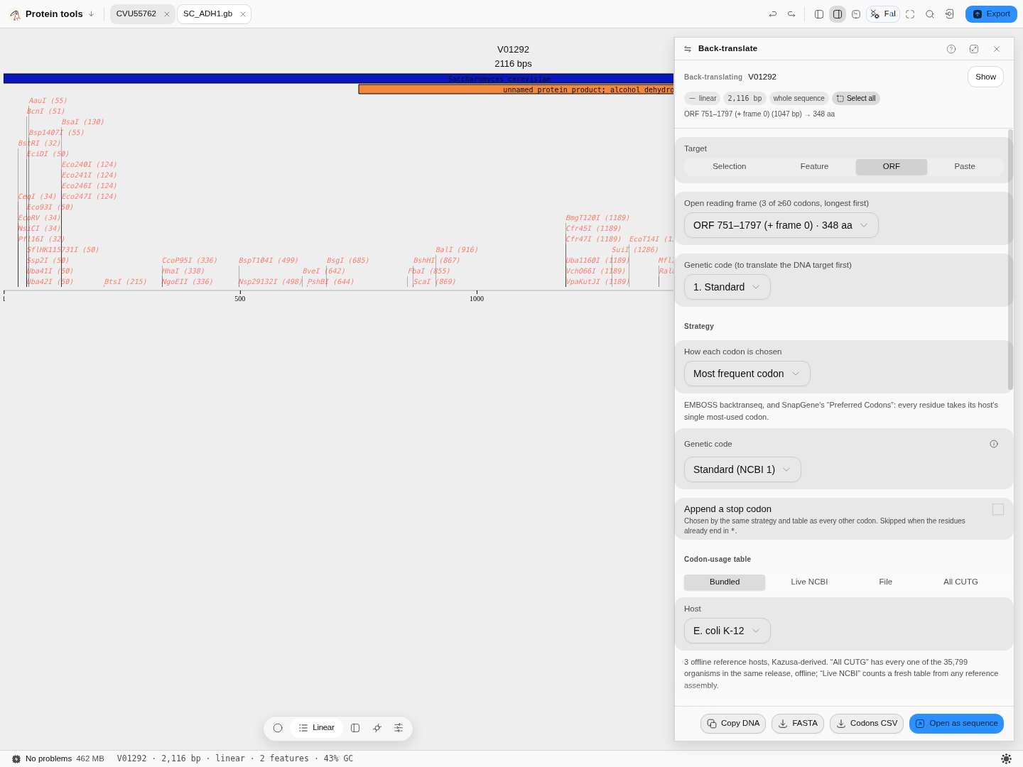 The ORF target on real yeast ADH1: the picker, the header and the product all agree that the 1047 bp
frame yields 348 amino acids. The rule, the genetic code and the codon-table source are each a
control, and the blurb under the rule says what it does.
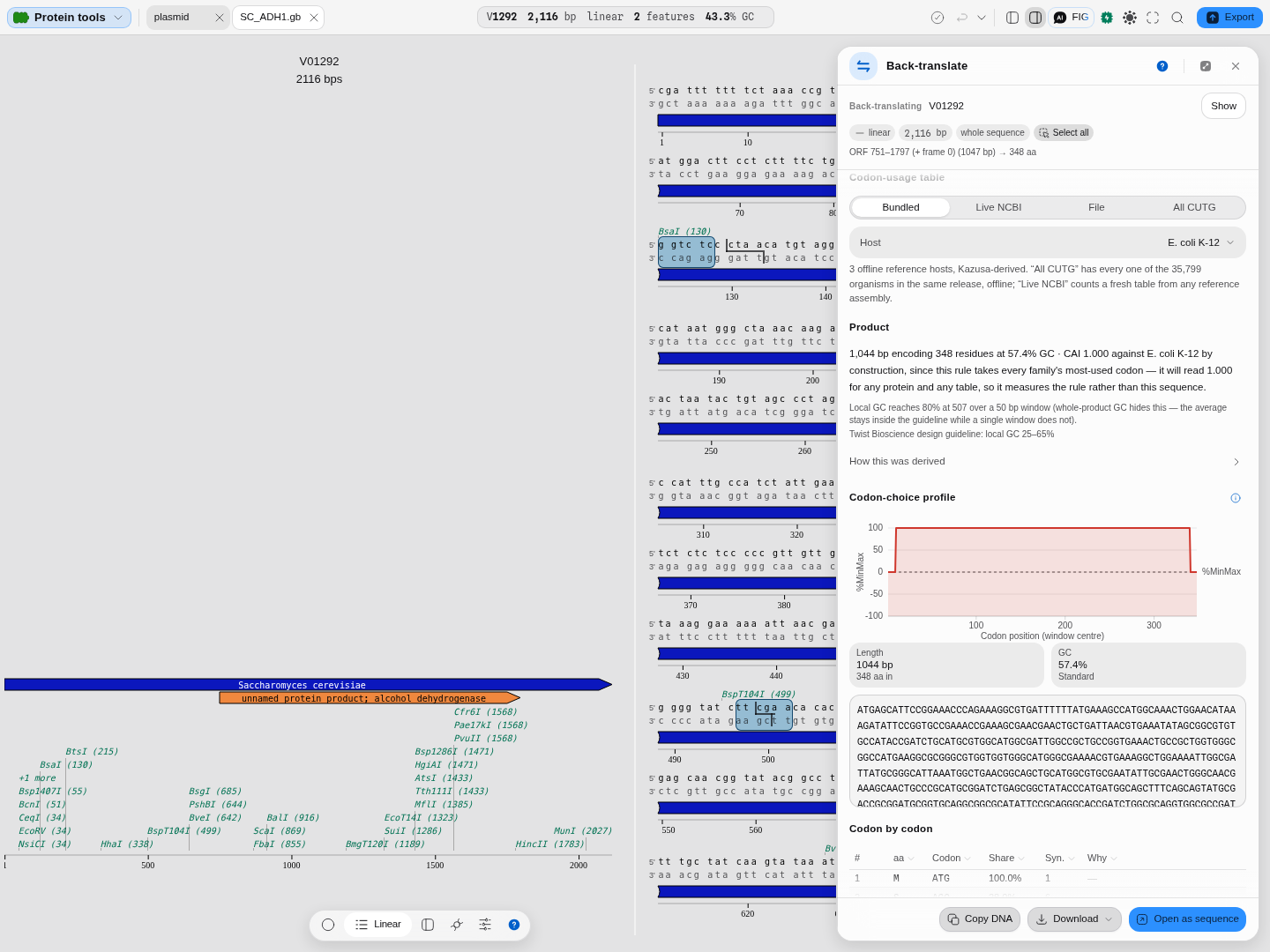 A real E. coli table loaded from file. The readout states what was read — 64 codons, 2,330,943
codons counted, 8,087 CDS — and says which of those figures the file published and which were counted
on load. The product below is 1044 bp at 43.8% GC.
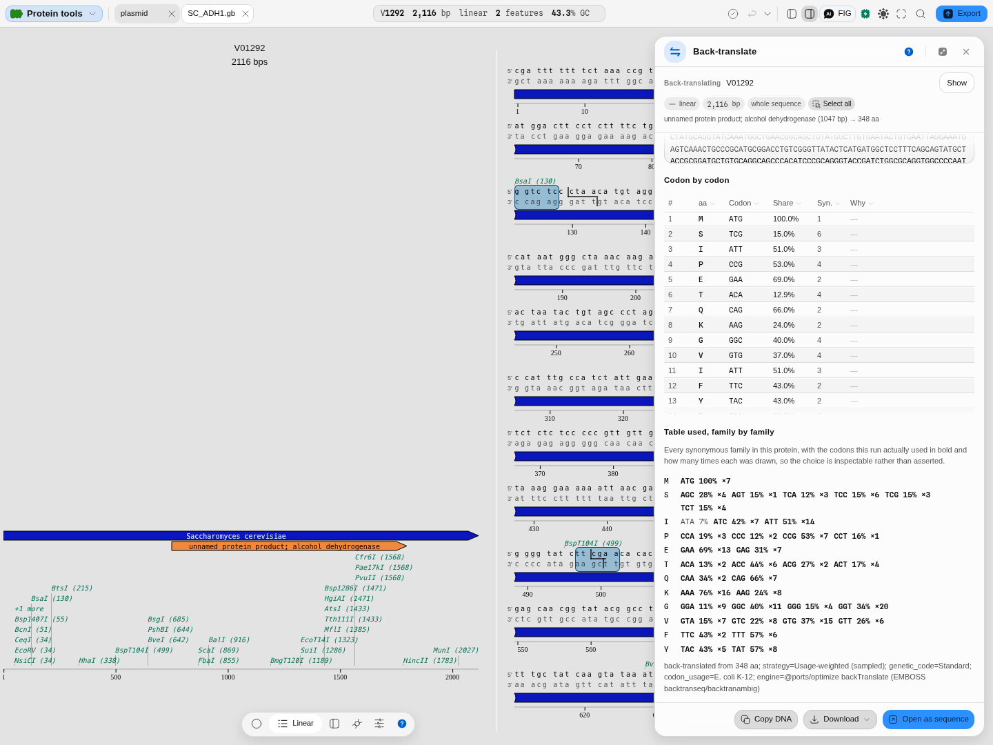 Under the usage-weighted rule, serine resolves to all six of its codons, each shown with the number
of times this run drew it. Under most-frequent-codon the same table shows one codon per family.
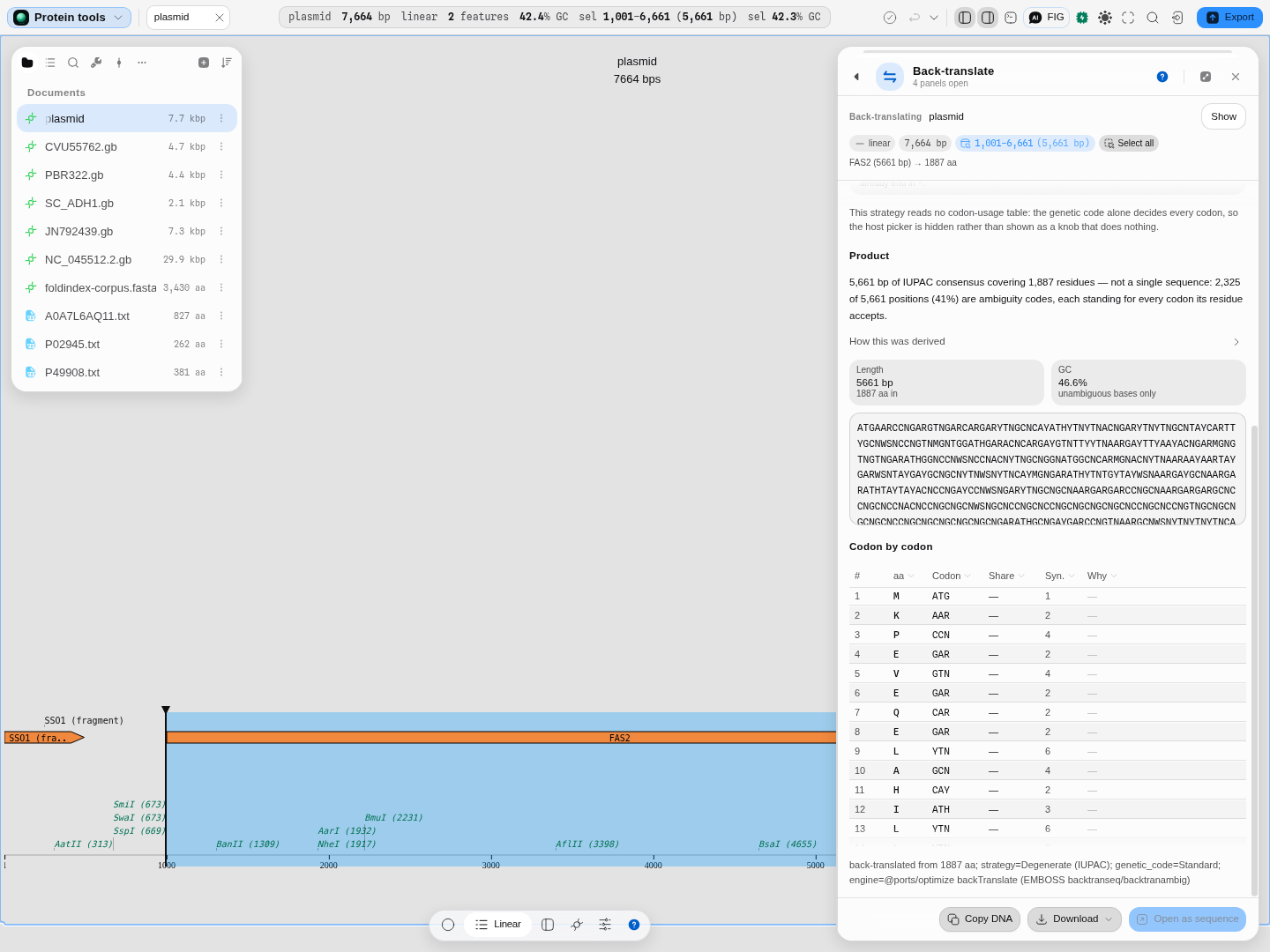 Degenerate (IUPAC): "Open as sequence" is disabled with the reason stated next to the rule that
caused it, the host picker is hidden rather than shown as a control that does nothing, and GC is
labelled as counting unambiguous bases only.
Related
Feeds it: Protein Analysis hands its target straight here.
Follows it: Codon Optimization takes the product and applies real constraints — this is the intended next step for anything you plan to order. Codon Usage Analysis scores the result against a reference table.
Alternative to it: nothing else here goes protein → DNA. Going the other way is translation, on the sequence map.
In this group: Codon Optimization · CRISPR Guide Design · Genetic Circuit · In-Situ Probes · CRISPR Edit Inference · RBS & Operon Design · Barcode & Index Design · Auto-Annotate · Apply features from a file · Power and sample size: replicates needed to detect an effect, or the power a design has · Trade-offs: which candidates in a table are not beaten on every objective at once