
Codon Optimization
Marked experimental: the surface can change.
Rewrite a coding sequence for expression in a chosen host while holding the constraints that matter: forbidden restriction sites, GC window, homopolymer limits, and the encoded protein.
| Reached by | Tools → Codon Optimization |
| Sample project | Codon usage |
What it does
Codon optimization is usually sold as a lookup: swap every codon for the one your host uses most. That is one of the things this tool can do, and on its own it is rarely what you want — a gene made of nothing but optimal codons can fold badly, carry a runaway GC%, or acquire a restriction site that breaks the cloning plan you already have.
So this is a constraint solver, not a lookup table. You state what must stay true — the protein is unchanged, GC stays between 40% and 60% in every 50 bp window, no BsaI site anywhere, no run of more than 5 identical bases — and what you would like to be as good as possible, usually codon adaptation for a chosen host. The solver finds a sequence that satisfies every constraint and scores as well as it can on the objectives, and tells you precisely which constraints it could not meet rather than silently returning its best guess.
When you’d use this
Used in: Optimize a coding sequence for expression in another host
Three experiments that end up here, and they want different settings:
1. You are ordering a synthetic gene for expression in a new host. Human gene, expressed in
E. coli. Optimize for the host, protect the protein, and add the constraints your synthesis vendor
charges you for: a GC window, no long homopolymers, no repeats. Route: pick the CDS → Use best
codon → add GC content with a window and Avoid patterns 8xA → Open optimized →
Primer design for the flanks.
2. You need a site gone without touching the protein. A BsaI site inside your insert is blocking
a Golden Gate assembly. You do not want the whole gene rewritten — add BsaI_site to Avoid
patterns, turn the codon objective off, and the solver makes the smallest synonymous change that
kills the site. Route: → Golden Gate.
3. You are matching a host's usage rather than maximising it. For a protein that folds co-translationally, the fastest possible translation is not the goal. Use Match codon usage or Harmonize RCA instead of Use best codon — see Algorithms.
Pro tip. If your gene is already in a plasmid you care about, optimize with the map showing Original, then flip to Optimized before you export anything. That one comparison catches the restriction sites an optimization silently created or destroyed — the failure that surfaces two weeks later at the ligation step.
The panel says what it will act on
The header of every tool panel names its target, and in the optimizer that is the region you picked, not whatever happens to be selected on the canvas — so a run targeted at a CDS keeps saying so after you click elsewhere, or reload the project a week later. Clicking the target chip selects that stretch on the canvas, which is the quickest way to see the span a set of coordinates actually refers to before you commit a solve to it.
Designing for expression: several answers, not one
The comparison is the point. Four published strategies disagree about what limits how much protein comes out, and the honest answer is to run them side by side rather than to pick one for you.
- Maximise codon adaptation — every amino acid takes the host's single most-used codon. The highest CAI you can reach, and the least like any real gene: uniform codon choice removes the translational pauses a nascent chain may fold around.
- Match the host's codon usage — reproduce the host's synonymous-codon distribution rather than its argmax, so rare codons stay at the rate they occur at naturally.
- Harmonise with the native host — put each codon at the same relative adaptiveness it had in the gene's original organism, so the elongation rhythm survives the transfer. This one needs the native host's codon table as well as the target's.
- Preserve the initiation region — recode nothing over the first bases of the message and optimise only downstream.
Each design comes back with its CAI, its GC, the folding free energy of the initiation region, a rare-codon count if you asked for one, and how many bases it changed. The comparison, the strategy each answer followed and what it trades away can be saved into the project as a document, so the reason you chose one is still there six weeks later.
Why the initiation region gets its own strategy. Kudla and colleagues built 154 versions of one GFP gene that differed only at synonymous sites, and saw protein levels vary 250-fold. Codon bias did not correlate with expression; the folding free energy of the message over nucleotides −4 to +37 around the start codon explained more of the variation than any other predictor, including CAI. That window is the one reported here, and it is worth watching: on a real yeast gene redesigned for E. coli, all three recoding strategies made it more structured than the untouched sequence.
And a high CAI is not a high titre. A 2025 comparison of codon-optimization tools reports CAI correlating negatively with titre in some settings. The number is reported; the claim is not made.
What this computes
A constraint solver's answer, and what it could not satisfy — never a lookup table's guess.
-
The optimized sequence, and which bases changed: the edit count and the runs of changed positions, so the diff is inspectable rather than implied
-
Every constraint, before and after, row by row — with
successfalse and the solver's own message when a hard constraint could not be met, rather than a best guess returned as an answer -
Every objective, before and after, and the weighted objective score either side, which is the optimization delta
-
GC before and after, and CAI before and after — null, not zero, when there is no codon table or the length is not a multiple of three, because a missing measure and a measure of zero are different facts
-
Alternatives, when you ask for them: several solutions from one base seed, each with its own seed, sequence, edit count, GC and CAI, plus how many are actually different sequences. One distinct answer means the problem has one answer, not that the run failed
-
The seed the run used, echoed back — and null when it was unseeded, because an unseeded run is not reproducible and nothing on screen may imply that it is
-
For an expression design: one sequence per strategy, each with its codon adaptation index, GC fraction, initiation-region folding free energy over the Kudla window, rare-codon count where you set a threshold, edit count and fraction of codons changed — plus the untouched sequence scored the same way, so "did this improve anything" is answerable from the table. Every one of those numbers names the model that produced it and the codon table it was computed against, and a strategy that could not run is named with its reason rather than quietly leaving the table one row shorter
-
Every cryptic splice site the sequence spells: each
GTandAGwith its position and strand, the window that was scored, its maximum-entropy strength and its typicality against measured Arabidopsis splice-site frequencies — two numbers on two different scales, reported separately and never combined, with no threshold and no verdict, because neither model publishes a cutoff -
Where the design shares sequence with anything else you name, which is the orthogonality question: for each shared window, its position in your design, how many single-base mismatches it tolerated, and whether it matched the forward or the reverse strand — both strands are always searched, because a site that anneals to the reverse complement is a site. Two readings of the same finding are available and they answer different questions: a fixed-width window report lists every window of the length you set, which is the right shape when you care about priming or recombination at a defined length; a maximal-stretch report gives each shared run once at its full length, which is what you want when the question is how much do these two molecules actually have in common. A shared stretch is reported at its true maximal extent, so a run that happens to continue one base past the length you asked about is reported as the longer number rather than truncated to your threshold
-
Whether the constraint was already satisfied by your original sequence, or repaired by the run — a distinction the tool draws for every constraint, because "satisfied" over a sequence the solver never had to change and "satisfied" after it rewrote the region are different claims about your design. A constraint the solver satisfied by construction is labelled as guaranteed rather than measured, and is never presented as evidence that your original bases complied
Mismatch tolerance is exact, and it is bounded at three. Windows are compared allowing zero to three single-base substitutions, and the count reported for a window is the fewest mismatches found anywhere it matches. Insertions and deletions are not part of this comparison. The maximal-stretch reading is perfect matches only; if you need to tolerate mismatches, the fixed-width reading is the one that does it, and asking the maximal-stretch reading for a relaxed identity is refused by name rather than approximated, because a relaxed identity makes the answer depend on an alignment heuristic rather than on the question.
Ambiguity never counts as shared sequence. A run of N matches nothing, including another run
of N — two records that are both unresolved in the same place have not been shown to have anything
in common. A non-ACGT position also breaks a shared window rather than costing a mismatch, so a
window cannot be reported as spanning one.
Seeding is reproducible inside this engine only. It does not reproduce the upstream library's own random stream, so a seeded run here will not match a Python run with the same seed, and the tool says so rather than implying cross-language determinism.
Vendor limits: will the supplier make this?
A separate check on the same sequence, answering the question the rewrite is for. It measures the sequence against what a named synthesis vendor publishes it can make, and every threshold is that vendor's own, carrying the page it was read from and the date it was read:
- length, against the range the product is offered in
- average GC across the whole sequence
- GC in a sliding window, where the vendor states one — this is the measure that catches a design whose overall composition is fine and whose local stretch is not, and it is usually the first one a real sequence fails
- the longest homopolymer run. Some vendors state one limit for all four bases; others state a different limit for A/T than for G/C, and both are kept as stated, because flattening them to the stricter over-reports on an AT-rich design and to the looser misses a real problem
- the longest short tandem repeat, for the unit sizes the vendor names
- the longest repeat of any kind that occurs more than once, and the longest inverted repeat — the hairpin-forming arm
Every limit is reported, met or not: a list of failures alone cannot tell a clean sequence from an unchecked one. Each exceeded limit that has a position carries it, and those are drawn on the map so a 34 bp homopolymer is somewhere you can go rather than a number. Length and average GC are properties of the whole record and have no position, so they are never drawn — and the panel says so rather than leaving you looking for a mark.
A limit a sequence cannot be graded on is stated, not skipped. A 40 bp insert has no 50 bp window, so the windowed-GC limit does not apply to it — which is different from passing it, and silence would make the shorter sequence look like the cleaner one.
Two vendors can honestly disagree about one sequence, and that is the reason this is a profile per product rather than a single verdict: a 12-base run of A is over one supplier's published limit and inside another's.
What it is not. It is not a prediction that synthesis will succeed, and it is not a refusal. A vendor publishes what it supports; a sequence outside that envelope is a conversation with the supplier — often a different product, a higher complexity tier or a longer turnaround — rather than a rejection. Nothing here contacts a vendor, and no sequence leaves your machine.
Cryptic splice sites: did the rewrite spell one?
The check this panel makes necessary. Optimisation chooses synonymous codons for codon usage, GC and the vendor's limits — and none of those objectives knows what a spliceosome reads. A swap can spell a strong splice donor that was not there before; the gene then looks correct in a tube and is spliced somewhere nobody intended once it is in the organism. In a plant host this is a common and expensive way for an optimised transgene to fail.
Every GT and every AG in the sequence is found and scored two ways, which are deliberately
not on one scale and are never added together:
- Strength — how much the surrounding bases look like a splice site under the published maximum-entropy model (Yeo & Burge, 2004), the same model MaxEntScan uses. It is a log-odds score in bits: higher means more site-like.
- Typicality — how much they look like a real splice site in a plant, scored against base frequencies counted at the annotated splice sites of Arabidopsis thaliana (TAIR10, Ensembl Plants release 63 — 256,158 introns). Also in bits, against a different background.
Why both: the first says "this is a strong site", the second says "this is the kind of site this organism actually uses", and a sequence can score high on one and not the other. Keeping them in separate columns is what lets you tell those cases apart.
It ranks; it does not call. There is no threshold, no flag and no red badge, and that is not an omission: neither the published model nor the measured frequencies comes with a significance cutoff, and inventing one would be a judgement dressed as a measurement. The candidates are sorted strongest-first and both numbers are shown; whether a given site is worth designing around is yours to decide — usually against the rest of the construct and the host you are going into.
Which strand is read. Both, by default: a site on the antisense strand still splices any transcript made from that strand, and in a construct both may be transcribed. Select a gene or mRNA on the map first and the scan reads that gene's own strand instead, saying so under the control; the other strand's candidates then stop competing for places in the ranked list. On the human EMX1 locus that moves three of its five annotated intron edges into the top fifty, where both strands together left two. Pick another strand to override it.
Why the frequencies are plant ones, measured here rather than borrowed. The mammalian 3′ splice site carries a polypyrimidine tract — C and T together — while Arabidopsis is markedly T-rich at the same positions. That is a different distribution, not a small difference, so scoring a plant sequence against human matrices would be the wrong comparison. The matrices are counted from a named assembly at a named release, and the count is reproducible: the same release gives the same numbers.
Where it lives
Tools → Codon Optimization, or right-click a CDS on the map and use the Optimize submenu, which arrives already scoped to the feature you clicked. It opens in the right rail beside the sequence, so the map stays visible while you work — which matters, because the map is half the readout.
Inputs and outputs
In: one region of the open sequence — the whole thing, your current selection, or a coding feature picked from a list (the picker shows each feature's length and warns when it is not a multiple of three). Plus a codon-usage table for your host.
Out: a sequence of exactly the same length, a per-constraint pass/fail report, the CAI and GC shift, a per-codon list of what changed, and two profile plots. Nothing is written to your open file until you ask: Open optimized creates a new document, GenBank downloads one, and CSV / PDF export the report.
Pro tip. Optimization never changes length, by construction. That is why every feature on your plasmid keeps its coordinates and why the before/after profiles line up base-for-base with the ruler — and it is also why a length constraint can only ever verify, never fix.
Demo
Not recorded yet. A screencast belongs here and does not exist. The worked example below is a real run on a bundled starter, reproducible number for number — and, when you set a seed, literally reproducible.
Worked example
Open the PCR, multiplex & fusion sample project. It arrives loaded with pBR322, a 4,361 bp
cloning vector carrying two well-known coding sequences: tet (tetracycline resistance, 1,191 bp)
and bla (β-lactamase, 861 bp).
- Open Codon Optimizer and set Target to
CDS: tet (1191 bp). The panel selects the region on the map as you pick it, so you can see what you are about to change. - Leave the codon table on the bundled E. coli K-12 reference. (The Live from sequence option is offered but refuses here, and says why: pBR322 is an artificial vector, and there is no reference assembly to count real codon usage from. Pick the expression host you will actually use, not the plasmid.)
- Keep Codon optimization → Use best codon (max CAI) and Protect protein on.
- Press Optimize.
The run replaces 260 bases — every one a synonymous change, so the protein is untouched:
| Before | After | |
|---|---|---|
| Codon Adaptation Index | 0.604 | 1.00 |
| GC content of the region | 61.5% | 64.9% |
| Constraints satisfied | — | all |
A CAI of 1.00 means every codon in the gene is now the most-used codon for its amino acid in the chosen host. That is the maximum the objective can reach, and it is worth knowing that it is also an extreme: real highly-expressed genes rarely look like this, and stretches of identical codons can create their own problems (see Limitations). The codon quality histogram under the result shows the whole distribution shifting rather than a single average, and the CAI profile shows which stretch of the gene was dragging the number down before.
What optimization costs you elsewhere in the plasmid
Rewriting 260 bases inside a gene changes more than that gene's codons — it silently creates and destroys restriction sites, which is what breaks a cloning plan two weeks later.
Set Showing on map to Optimized and the canvas redraws over the new bases: the plasmid map,
the sequence view, the translations and the cut sites are all recomputed from the optimized
sequence. On this run, inside tet:
- Lost:
PshAIat 717,BveIat 1055. - Gained:
BveIat 613,FbaIat 1076.
Switch back to Original and the document's own bases return. Switching costs nothing and never re-runs the solver — it is the same result, drawn over a different sequence.
While the optimized bases are on screen the document is read-only, and your saved project always keeps the original sequence. The optimized version becomes a real sequence only when you ask for it: Open optimized creates a new document, and GenBank downloads it. Nothing you preview is saved on top of what you started with.
If a site you rely on disappears, you do not have to accept it: add it as a region pin — Enforce sequence over the site's coordinates — and run again. The solver will optimize around it.
Reading the result
A finished run reports more than a sequence, and three of its readouts answer questions that a single "all constraints satisfied" line cannot.
A green tick means one of three different things
Every constraint is evaluated twice: once against the sequence you started with, once against the one the solver produced. What the panel puts beside a satisfied constraint says which of these happened.
| Label | What it means | What you can conclude |
|---|---|---|
| repaired by this run | Your original sequence breached the constraint; the run fixed it | The edits under this constraint are real changes you asked for |
| already satisfied | The constraint was measured against your original and held | Nothing here needed changing |
| guaranteed, not measured | The solver only ever allowed bases that satisfy it, so it was never tested against your original | Nothing at all about your original sequence. The run may have rewritten every base in its span |
The third one matters more than it looks. Constraints that fix bases directly — an Enforce
sequence pin, an initiation-context motif — are satisfied by construction: the solver builds them
into the space of sequences it is allowed to consider, so asking "did the original pass?" is a
question it never has to answer. Pinning CAAAACATG over a stretch reading GGGGGGATG is reported
as satisfied before the run and then changes six bases. Read the Edits count and the amber
marks on the map, not the tick, to see what actually moved.
Edited bases and amber runs are two numbers
The result reports the number of edited bases, and the map draws contiguous runs of them.
A run of three adjacent changes is one amber mark over three bases, so the two numbers rarely
match — on a typical bla optimization, 203 edited bases draw as 175 runs. The panel names both
rather than showing one number twice.
Objectives, one row each
Under the aggregate objective score, every objective gets its own before-and-after row, with its weight when it is not 1. With a single objective the aggregate is enough; the moment you combine two — codon optimization plus an initiation-strength target, say — the total can improve while one of them goes backwards, and only the per-objective rows show it.
Was this run reproducible?
The panel reports how many random draws the solve made, not just a verdict. Zero draws is a proof rather than an estimate: no randomness was consumed, so re-running with any seed returns exactly this sequence and Re-roll cannot produce an alternative. That is the usual case for objective-driven runs. Constraint-driven runs — a GC window plus a forbidden pattern, for instance — do draw, and there Alternative solutions gives you genuinely different sequences that satisfy the same requirements. When draws happened, compare the candidates rather than assuming they differ.
Controls
Target region — whole sequence · current selection · a coding feature. The badge next to it tells you the length and whether it is in frame.
Read on — which strand the reading frame runs along. A gene annotated complement(3293..4153)
is transcribed from the bottom strand, so its codons exist only in the reverse complement of the
bases you see on the map. Pick that feature and the panel says so — "861 bp · circular · reverse
strand", and "read 3′→5′ on the bottom strand" — and every codon-level option runs in the gene's
own frame. A whole-sequence or selection target has no annotated strand of its own, so this control
is where you say which one you mean; a feature target uses the strand the record gives it.
Why this is not a detail. Optimizing a reverse-strand gene on the forward strand is not a slightly worse answer, it is a different gene: the forward bases of bla in pBR322 translate to a protein that stops at residue 7. Protect protein would faithfully protect that nonsense while reporting success.
Codon-usage table — a bundled reference host, a table computed live from the record's own organism, a codon-usage file you upload, or any of the 35,799 organisms in the CUTG release. If the record is a cloning vector the live option refuses and says why: an artificial sequence has no reference assembly to count usage from, so pick the host you will actually express in.
Objective — the codon-optimization method, with a weight.
Constraints, each independently switchable and parameterised:
| Constraint | What it holds | Typical use |
|---|---|---|
| Protect protein | The translation is unchanged | Always on, unless you mean to change the protein |
| GC content | A percentage band, optionally per window | Synthesis vendor limits; a window catches local extremes a global bound misses |
| Avoid patterns | Any DNA/IUPAC string, 8xA homopolymers, or an enzyme name like BsaI_site | Removing sites, depleting motifs, killing repeats |
| Avoid rare codons | No codon below a frequency you set | Blunter than the CAI objective, and a hard rule rather than a preference |
| Avoid hairpins | Stem length and window | Secondary structure that stalls translation |
| Unique k-mers | No repeated k-mer | Synthesis difficulty; assembly mispriming |
| Terminal GC | GC bounds on the two ends only | The vendor constraint on primer-binding ends |
| Length bounds | Verification only | Checking a region fits a synthesis order |
| Avoid motifs (PSSM) | No window scoring above a threshold on a position-weight matrix | Transcription-factor binding sites, and any motif that is a score rather than a string |
The named controls, in the order the panel shows them
| Control | Default | What it sets |
|---|---|---|
| Host | E. coli K-12 | The reference organism the codon-usage table is taken from, including any table you saved |
| Basis | Highly-expressed genes | Whether the table counts highly-expressed genes or every annotated CDS in the reference assembly |
| Genetic code | Standard | The translation table the protein is read under |
| Strategy | Use best codon (max CAI) | Also Match host codon usage and Harmonize RCA |
| Boost | 1 | The weight this objective carries against the others |
| Original host | none | For harmonization, the organism the gene came from |
| Count rare codons | off | Reports how many codons fall below a within-family frequency. It adds no constraint, so the designs are unchanged by it |
| Terminal GC bounds | on | GC limits on the two ends only, the constraint most synthesis vendors apply |
| Anchor CDS | none | Which coding feature the ribosome-binding site is designed ahead of |
| Pattern to avoid | empty | A DNA or IUPAC string, a homopolymer such as 8xA, or an enzyme name |
| JASPAR matrix id · Motif name | empty | The position-weight matrix a window is scored against, and what to call it |
Pinned regions
| Control | What it sets |
|---|---|
| Compatibility | What a set of pinned regions must satisfy together: Differ by at least N bases, or a usable Type-IIS junction set |
| Enforced sequence | The exact bases this span must end as. IUPAC accepted, and it must be the span's length |
| Allowed choices | A pipe-separated list of alternatives, each the span's length |
| Pattern and count | A site, a sequence or an enzyme name, and how many times it must occur |
| Avoid matching | Sequences this span must not match |
| Other primers | Primers this span must stay distinguishable from |
Avoiding a binding site, which is not a string
A restriction site is six fixed bases; a transcription-factor binding site is not. TP53 does not bind one sequence, it binds anything that scores well enough on a matrix built from hundreds of observed sites — so "remove the TP53 sites" is a question about a threshold, and a pattern field cannot ask it.
Two ways to give the tool a matrix:
- A JASPAR id — type a versioned id such as
MA0106.1and press Fetch. The matrix comes from JASPAR live, so a run always uses the current release rather than a copy that went stale. The version after the dot is required, because a matrix is revised between releases and the scores change with it. - Your own aligned sites — paste them one per line, all the same length, and the tool counts them into a matrix. This is the right answer for a motif no registry has: a SELEX result, a designed operator, or the sites annotated in the record in front of you.
The threshold is a percentage of the matrix's own score range, so it means the same thing for every motif: 90% is a strict site, 70% catches weak ones. Lower it and you will find more sites and give the solver more to do — a short motif at a low threshold can easily be unsatisfiable while the protein is protected, and the panel says which constraint it could not solve and where.
The consensus shown beside each motif is for reading, not matching: upper case where the top base holds at least half the counts in that column, lower case where it does not. The matching is done on the matrix.
Designing the ribosome-binding site
In bacteria the start codon's context is not a consensus at all — the ribosome finds the start by pairing a Shine-Dalgarno sequence in the 5′UTR with the 3′ end of the 16S rRNA, and how strongly it initiates depends on that pairing, on how far the site sits from the ATG, and on whether the mRNA folds the whole thing up. RBS strength puts that calculation inside the solve, so the optimizer can design a 5′UTR toward an initiation strength rather than hand you a number afterwards.
Point it at a start codon, choose at least or target, and give it a relative strength. Three
things it checks before it will run, each with the reason on the control:
- the start codon has to be inside the target region;
- the gene and the region have to be read on the same strand, or the "5′UTR" would be downstream of the ATG;
- there has to be enough 5′UTR inside the region — roughly 30 bases — for a Shine-Dalgarno site to sit in at all. A CDS-only target has none.
Pro tip. Asking this over a whole circular plasmid is the expensive way: a circular problem is solved on a tripled view, so the folding runs three times over. A selection spanning the 5′UTR and the first part of the gene answers the same question much faster, and it is the region you actually want the solver rewriting.
It is an objective rather than a hard constraint on purpose: an unreachable target still gives you the best 5′UTR the solver found, where a hard band would fail the whole run.
The start codon's context
A scanning ribosome does not recognise ATG alone — it reads the bases around it, and the strength
of that context decides how often the start codon is used. Translation-initiation context, under
Region pins, places the surveyed consensus around a start codon you choose:
| Context | Consensus (5′→3′, IUPAC) | Derived over |
|---|---|---|
| Vertebrate (Kozak) | GCCRCCATGG | 699 vertebrate mRNAs |
| Higher plants | CAAMAATGGCG | 5,074 plant genes |
| Dicot plants | AAAMAATGGCT | dicot angiosperm mRNAs |
| Monocot plants | CMRMCATGGCG | monocot angiosperm mRNAs |
| Drosophila | CAAAACATG | Drosophila nuclear genes |
The purine at −3 is the most conserved position in the vertebrate motif — 97% of mRNAs have one, usually A — and G at +4 is the second determinant. Plants put purines at both positions in about 80% of mRNAs, more often at +4 and less often at −3 than vertebrates do. Drosophila differs from vertebrates upstream of the start codon but behaves identically at that −3 position, which is the survey's own conclusion: the mechanism is shared and the flanking preference is not.
The Drosophila motif ends at the start codon, so unlike the vertebrate and plant contexts it
constrains nothing downstream of ATG and can never collide with Protect protein. If you are
expressing in S2 cells or designing a fly transgene, that makes it the one context you can pin on a
coding region without checking residue 2 first.
Two things the panel will tell you before you pin anything, because both are easy to walk into:
- The motif sits upstream of the ATG, so it cannot be inside a CDS-only target. Set the region to the whole sequence, or to a selection that includes the 5′UTR, and the pin has somewhere to live. Pinned against a CDS-only target it would simply be dropped.
+4 = Gconstrains the second codon. Only Ala, Gly, Glu, Asp and Val have codons beginning with G, so if residue 2 is anything else the motif and Protect protein cannot both hold. The panel names the residue and its codon rather than letting the solver discover it as a failure with no explanation.
There is no bacterial row here, and that is the right answer rather than a gap. Bacteria do not scan; that question is thermodynamic, and RBS strength above is where the optimizer answers it.
Region pins apply a constraint to a sub-span rather than the whole region: force exact bases, forbid changes, require a pattern, hold a Tm window, make a span primer-friendly, keep it from cross-dimerising with a primer pool, or hold a whole set of spans compatible with one another. Each pin carries its own priority and weight.
Pro tip. A pin that misses your target region is reported on the card rather than silently ignored — but it is easy to create one by pinning coordinates from a different sequence. Pin from a selection where you can.
Keep a set of regions compatible with each other
Every other pin judges one span on its own. This one judges spans against each other, and it is the pin to reach for whenever your design contains several stretches that have to stay different — assembly junctions, barcodes, landing pads, spacers, primer sites — while the optimizer is free to rewrite the sequence around them.
The pin's own span is the first region of the set; the rest you type as start-end, one per line,
or push in from the canvas with Add selection. Then pick the rule the set has to obey:
| Rule | What it asserts | Reach for it when |
|---|---|---|
| Differ by at least N bases | no two regions may differ at fewer than N positions | keeping a set of tags, spacers, barcodes or landing pads apart, so nothing recombines or mis-primes between them |
| Usable Type-IIS junction set | no two regions may be identical or reverse-complementary, and none may be palindromic | designing where a Golden Gate assembly will be cut, so the fusion sites cannot mis-ligate, cross-ligate or self-ligate |
| Do not cross-dimerize | no two regions may anneal to each other above a melting temperature you set | several primer or probe sites inside one construct that must not find each other |
The junction rule is the same rule the Golden Gate fidelity readout applies to fusion sites, so what the two tools call "a usable junction set" cannot drift apart. The difference is what you can do about it: the fidelity readout tells you whether the overhangs you already have are sound, while this pin makes "stay sound" a constraint the optimizer designs toward — you get a sequence that is codon-optimized, GC-bounded, site-free and still cuts into a junction set that assembles.
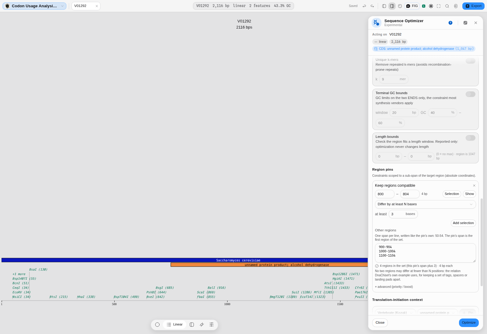
Every region must sit inside your target region, and the panel refuses rather than trimming. A span that hangs outside would be quietly shortened, and a shortened span is a different question: under Differ by at least N it compares fewer bases and can pass where the span you meant would fail. Under Differ by at least N all regions must also be the same length, because the rule compares them position by position; the panel names the lengths it found when they are not.
Step by step
- Open a record and pick a target region — for the walk-through below, the alcohol dehydrogenase CDS of the yeast ADH1 record in the Codon usage starter (1,047 bp).
- Under Region pins, choose Keep regions compatible and press Pin. The card appears with your current selection, or the whole region, as its span.
- Set the span to the first region you care about —
800–804here. - Type the rest into Other regions, one per line:
900-904,1000-1004,1100-1104. The line under the box confirms what it read: 4 regions in the set (this pin's span plus 3) · 4 bp each. A line it cannot read is named back to you rather than dropped, because a dropped line is a region you believe is constrained and is not. - Pick the rule. Leave it on Differ by at least N bases and set at least to
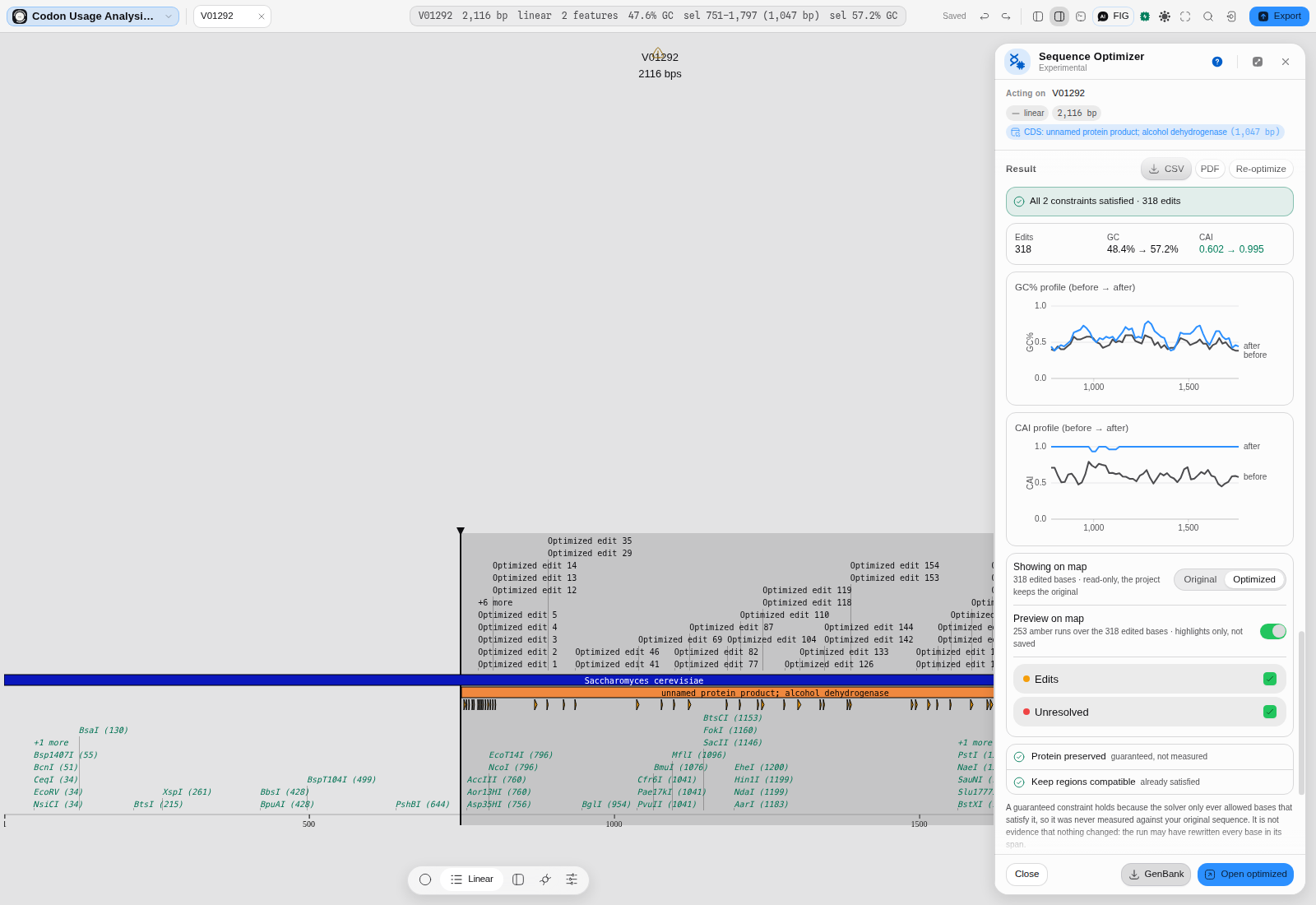
3— no two of these four-base junctions may share more than one base. - Press Optimize. On this record the run satisfies both constraints and makes 318 edits, taking CAI from 0.602 to 0.995 and GC from 48.4% to 57.2%, and the constraint list reads Keep regions compatible · already satisfied — the four spans were far enough apart to begin with, and the optimizer kept them that way while rewriting the codons around them.
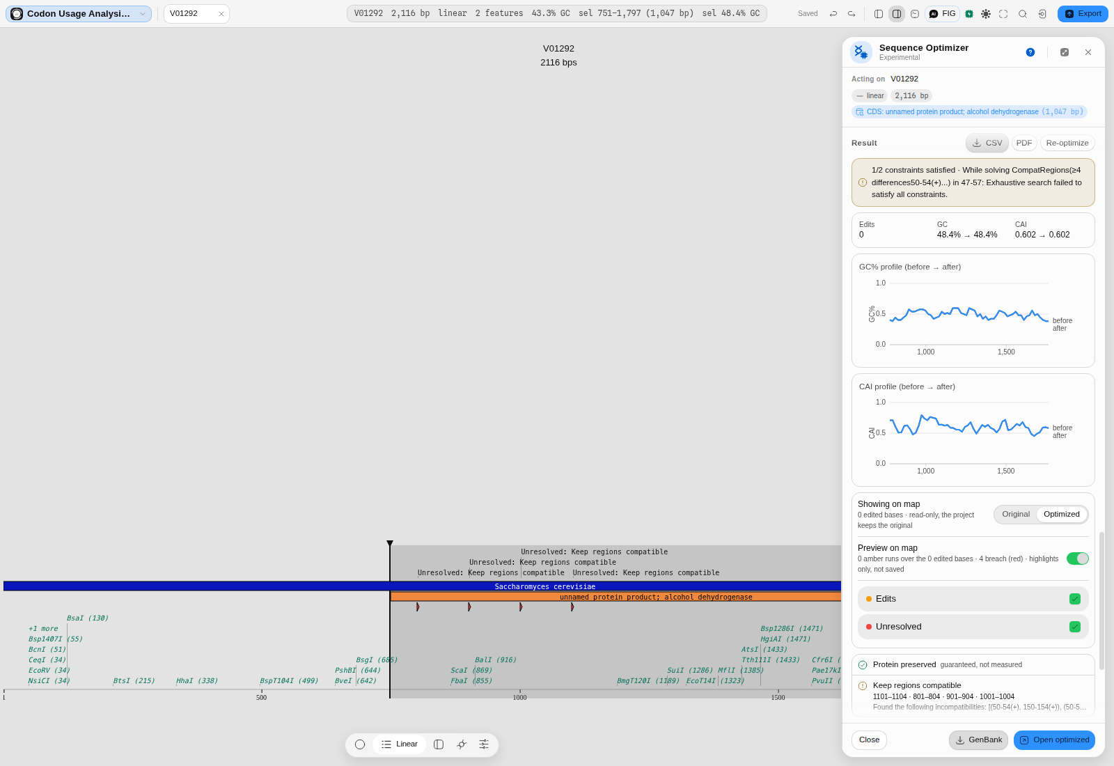
When it cannot be done, it says so and shows you where
Raise at least to 4 — demanding that all four bases differ in every pair — and the same run
comes back with 1 of 2 constraints satisfied and 0 edits. That is the honest answer, not a
failure to try: with Protect protein on, the solver may only make synonymous changes, and no
synonymous rewriting of this coding sequence can drive four four-base windows to complete mutual
difference.
What you get instead of an empty table is the diagnosis. The panel lists the pairs that clash, gives
their positions in the coordinates you typed (801–804 · 901–904 · 1001–1004 · 1101–1104,
ordered by how many conflicts each is in, fewest first), and — with Preview on map on — draws
each offending region in red on the sequence, so you can see which junction to move rather than
guessing. Move one span, loosen the rule by a base, or relax Protect protein, and re-run.
Cross-dimerization is judged with the same engine the primer constraints use. Pick Do not
cross-dimerize, set a ceiling in °C, and every pair of regions is scored with primer3's thal
duplex model — the same one behind No cross-dimer and Make primer-friendly, so a number here and
a number there mean the same thing. On the yeast ADH1 coding sequence, three 20-base stretches at a
0 °C ceiling come back repaired by this run: they did interact in the original sequence, and
the optimizer moved them apart while keeping the protein and improving CAI from 0.602 to 0.998.
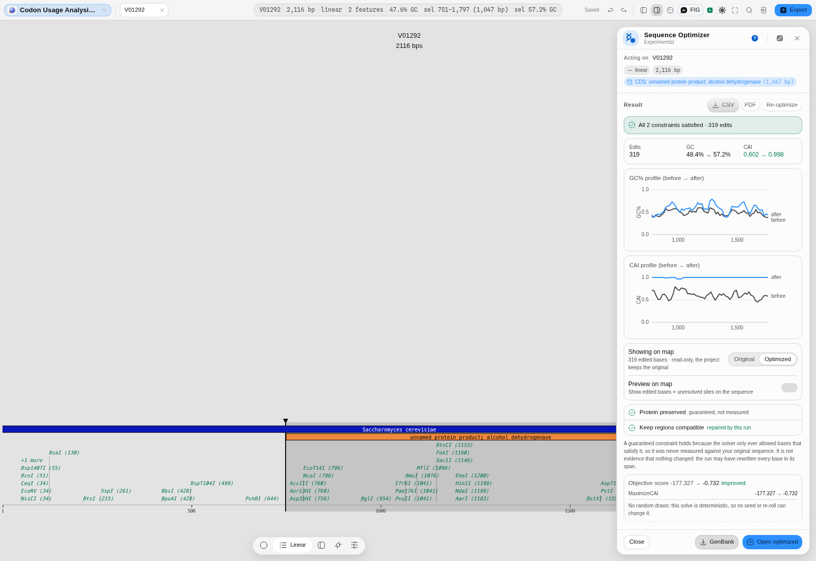
Read the tick, not just its colour. repaired by this run means the rule was broken in your starting sequence and the optimizer fixed it. already satisfied means it held before you ran anything. guaranteed, not measured means the solver could only ever produce sequences that obey it, so it was never checked against your original — and that is not evidence your bases were already fine.
Pro tip. The set always includes the pin's own span. If you want N regions compared, type N − 1 of them into the box — the confirmation line under it does that arithmetic for you, so trust the line rather than counting the rows you typed.
A pitfall worth naming. Differ by at least N on regions of different lengths is not a stricter or looser question, it is an undefined one, and the panel refuses it up front rather than answering something you did not ask. The junction and cross-dimer rules compare whole stretches rather than positions, so they take mixed lengths happily.
Two pins that ask for the same thing, and two that ask for opposite things
These are different situations, and the panel treats them differently on purpose.
The same pin twice is one pin. A constraint is defined by its kind, its span and what it demands, so pinning an identical one again asks the solver for nothing new — it is the same requirement stated twice, and a solver that satisfies it once has satisfied it. The panel says so and adds nothing, rather than leaving you two identical cards to tell apart later.
Two pins demanding different bases at the same position cannot both be met, and that is worth
catching before you spend a solve on it. It is easy to walk into with the initiation-context preset:
pin the vertebrate consensus around a start codon, then pin the Drosophila one around the same
codon, and you have asked for GCCRCCATGG and CAAAACATG over overlapping stretches that disagree
from their first base. Both pins stay — you made both requests, and which to drop is your call — but
the panel names the exact base where they collide, so you can see which one to remove.
Ambiguity codes are read as the sets they stand for, not as letters. R (A or G) and A agree; R
and Y (C or T) cannot, because no base satisfies both. That is why a consensus written with R,
Y or N will often coexist happily with an exact pin that a naive character comparison would
have called a clash.
Vendor limits
| Control | What it changes |
|---|---|
| Vendor | which product's published limits to measure against. Each carries its own numbers, and two can disagree about one sequence |
| Sequence | what to measure: the open record by default, a project document, or the current selection |
| Feature | measure a named feature instead of the whole record — the insert you are about to order rather than the vector it sits in |
Algorithms you can choose
Three codon-optimization methods, and they answer genuinely different questions:
| Method | What it does | When it is the right one |
|---|---|---|
| Use best codon | Every amino acid gets its host's most frequent codon | Maximum expression is the only goal. Drives CAI to 1.00 — see the caveat in Limitations |
| Match codon usage | Reproduces the host's distribution of codons rather than its argmax | You want a gene that looks like a native host gene, not a synthetic extreme |
| Harmonize RCA | Preserves the relative adaptiveness a codon had in its ORIGINAL host | Co-translational folding: it keeps the slow patches slow, so pause sites survive the move between hosts. Needs the original host as well as the target |
The Codon Adaptation Index reported before and after is the standard normalised CAI, and the codon-quality histogram shows the whole distribution rather than just the mean — a mean can improve while a handful of very rare codons remain, and the histogram shows that where the single number hides it.
The science
The solver, the specifications and the codon-optimization methods are a port of DnaChisel, and the port is checked against the real library rather than assumed: outputs are captured from a genuine DnaChisel run and asserted byte-for-byte, including the cases where upstream behaves surprisingly.
The codon-usage tables are real published data — the bundled reference hosts come from
python_codon_tables, the CUTG option reads the release's own distribution files, and a live table
is counted from real coding sequences of the organism you name. Nothing here is a hand-typed
frequency table.
Melting temperatures used by the Tm and primer-friendliness pins come from a port of primer3's thermodynamic engine, validated against the real one.
Position-weight matrices are read in JASPAR's own format and converted to log-odds with JASPAR's own pseudocount rule; the reader and the scoring are checked against Biopython and DnaChisel over every matrix in a cached JASPAR release, both the scores and the exact set of windows they match in a real plasmid.
The initiation-context consensus motifs are quoted from the surveys that derived them — Kozak's 1987 compilation of 699 vertebrate mRNAs, Joshi's 1997 survey of 5,074 plant genes, and Cavener's 1987 comparison of Drosophila with vertebrates — and each one is checked against the string its own citation prints, so a transcription slip fails rather than ships.
Contexts for other invertebrates and fungi are not offered, and the reason is the same standard: the compilation that covers the rest of the eukaryotic tree does not print its consensus in text we can check against, and inventing one would be worse than leaving it out. Yeast is a different case again — the published work is single-gene mutational analysis reporting at most twofold effects, so there is no surveyed consensus to offer. For a yeast gene, optimize codons against a yeast table and leave the start context alone.
Shared with other tools: Codon usage compares how every tool that does this chooses its method.
Limitations
A CAI of 1.00 is an extreme, not a target. Every codon in the gene becomes its host's most frequent one, which no natural highly-expressed gene looks like. It also concentrates tRNA demand and removes the translational pauses some proteins fold around. If your protein misbehaves after optimization, Match codon usage or Harmonize RCA is the first thing to try.
Length is fixed. The solver only substitutes synonymous codons — it cannot insert, delete, or change your protein. A length constraint therefore verifies, and never fixes.
Constraints can be unsatisfiable together. Ask for GC below 40% in a proline-rich region and no sequence can satisfy it. The report says which constraint failed and where rather than returning a best guess dressed as a solution, and the unresolved sites are marked in red on the map.
Off-target similarity is not checked. Two DnaChisel constraints that screen a design against a whole genome are not available here: they rely on BLAST or Bowtie running against a local genome index, which a browser cannot do. Use BLAST on the result if that matters.
When the run button is greyed out
Optimize refuses before it runs rather than after, and the reason sits next to the button. Five things stop a run, and each names what to change:
- No target. Pick a feature, make a selection, or take the whole sequence.
- The target is not a multiple of 3 while a codon-level option is on. Codons need a whole reading frame, so either point at a CDS or switch off Codon optimization, Protect protein and Avoid rare codons — the sentence quotes the length it measured, so you can check it.
- The RBS anchor cannot be scored — no start codon chosen, or one with no room for a Shine-Dalgarno site in front of it.
- A region pin does not validate — a pinned sequence whose length does not match its span, a pin running off the end of the record.
- A live codon-usage table has not been computed yet. The sentence names the organism a fetch would use — the one you picked, or the one the record itself names — so you can see what you are about to compute before you compute it. Fetch it, or switch the table to Bundled. This is the one that most often surprises people, and it is a deliberate refusal rather than a silent fallback: running anyway would score your gene against a table you did not choose. When the record names no organism at all the sentence says that instead of guessing one — a cloning vector is the common case, since pBR322's own organism is "Cloning vector pBR322", which has no reference genome, so pick your expression host yourself.
Finally, a run needs at least one objective or constraint switched on. With everything off there is nothing to optimize toward, and the panel says so rather than returning your own sequence back.
Compared with other tools
No first-party comparison has been made yet. Saying how this differs from IDT's, GenScript's or Benchling's optimizer would need their current documentation read and cited with a retrieval date, and that has not been done — so nothing is claimed here rather than something plausible being asserted.
What can be said without comparison, because it is a claim about this surface rather than about anyone else's:
- The constraints are the ones a synthesis order actually fails on, every one of them optional and parameterised — not a "strength" slider with the parameters buried behind it.
- A run tells you which constraint it could not satisfy, with the offending positions in your own coordinates and drawn on the map, instead of returning a best effort as though it were a solution.
- Constraints can be about how parts of the design relate to each other, not only about the sequence as a whole. Keep regions compatible asks a question a per-base or per-window constraint cannot express — "these four junctions must stay a usable set while you rewrite everything around them" — and it is the same junction rule the assembly tools apply, so a sequence optimized here cuts into an assembly that works.
- Twenty-two constraints and objectives are reachable from the panel, and the two that are not are listed with the reason, in a test that fails if a new one is added without a decision.
Export
Open optimized — the optimized sequence as a new document, carrying every feature from the original plus a marker over the region that changed. Your starting sequence is untouched.
GenBank — the same thing as a file.
CSV — DnaChisel's own before/after tables for every constraint and objective, plus the seed, so a run is reproducible.
PDF — a printable report of the same tables. It opens a print view; choose "Save as PDF" as the destination.
Pro tip. The CSV carries the seed. A constraint-driven problem can have many equally valid solutions, and the seed is what makes the one you chose reproducible — keep it with the order.
API
@ports/optimize — the solver, over plain strings:
import { optimizeSequence, optimizeCandidates } from '@ports/optimize';

const out = optimizeSequence({
  sequence, circular: false,
  constraints: [{ kind: 'EnforceGCContent', mini: 0.4, maxi: 0.6, window: 50 }],
  objectives: [{ kind: 'CodonOptimize', species: 'e_coli' }],
  codonUsageTable,            // required only when a codon spec is present
  seed: 1,                    // omit for the unseeded Math.random behaviour
  randomizationThreshold: 100 // see below — this is what makes alternatives real
});

// several alternatives at once, seeded from one base seed
const set = optimizeCandidates(input, { count: 3, seed: 1 });
The result is deliberately before-and-after in every field, not just the answer: success (all
hard constraints satisfied) or the solver's own failure message, nEdits and the edits as
half-open runs, constraintsBefore/constraintsAfter and objectivesBefore/objectivesAfter row
by row, the weighted objective score either side, gcBefore/gcAfter, and caiBefore/caiAfter
(null, not 0, when there is no codon table or the length is not a multiple of three).
seed is echoed back, and it is null when the run was unseeded — because an unseeded run is
not reproducible and nothing downstream may imply that it is.
randomizationThreshold is the knob that makes alternatives real. At DnaChisel's default of
10,000 essentially every localized sub-problem lands under the threshold, the exhaustive branch
runs, and the solve is deterministic — so "give me three candidates" returns three identical
sequences. Lowering it forces the genuinely stochastic mutation paths, which still satisfy the same
constraints while exploring different sequences.
Seeding buys reproducibility inside this engine only. It does not reproduce DnaChisel's numpy
stream: no seeded run here will match a Python run with the same seed=, and the port says so
rather than implying cross-language determinism.
Automation
- Workflow DAG: the node is
optimize_sequence, categorydesign, and a write node — it emits the optimized sequence as a new record, so downstream nodes act on the optimized molecule rather than the original, and it goes through the approval gate first. - Specifications are arrays,
constraintsandobjectives, each a list of DnaChisel specs —[{"kind":"EnforceGCContent","mini":0.4,"maxi":0.6,"window":50}]. That shape is load-bearing: the declaration once asked for an object, the runner read it withArray.isArray, and the call came back "provide at least one constraint or objective" with the caller having done nothing wrong. - Alternatives are first-class in the node too —
candidates,seedandrandomization_threshold— because "generate three and compare" was a thing only the panel could do until they were added, which is exactly the §10b asymmetry the two front doors are supposed to avoid. Candidate 1 is the plain unseeded answer; the rest run at seed+1, seed+2, … - Outputs:
record,sequence,success,nEdits,gcAfter,caiAfter(0 when not computable),candidates(each with its seed, sequence, edit count, GC and CAI) anddistinct— how many of the candidates are actually different sequences.distinct: 1means the problem has a single answer, not that the run failed, and it is reported rather than left to be inferred from three identical strings. - The copilot calls the same tool by the same name with the same parameters.
Provenance
A run is reproducible from three things, and all three are in the exported report: the codon-usage table you chose, the constraint set, and the seed. A constraint-driven problem often has many equally valid answers — the solver samples among them — so the seed is what makes the specific sequence you ordered the one you can regenerate.
Opening the result as a new document records where it came from, so the optimized sequence carries its origin rather than appearing as an unexplained file next to the original.
To describe the method in a paper: state the host codon-usage table and its source, the objective (max-CAI, match-usage or harmonize-RCA), and every constraint with its parameters. The CSV report is already in that shape.
The vendor limits carry their own provenance and it is not ours. Every threshold is the supplier's, read from the supplier's own published page, and the panel names that page and the date it was read beside the result. Nothing is averaged across vendors, nothing is inferred from a summary, and a vendor whose numbers could not be read at the source is absent rather than estimated — a missing profile is a legitimate answer where a guessed one would be a number with nobody behind it.
Screenshots
A set constraint alongside the per-sequence ones: four four-base junctions held at least three bases
apart while every codon around them is rewritten. The constraint row reads already satisfied —
they were far enough apart to begin with, and the run kept them that way.
The refusal, which is the more useful half: the rule cannot be met under Protect protein, so the
run says so, names the pairs in the coordinates you typed, and draws each offending region in red
rather than handing back a best effort.
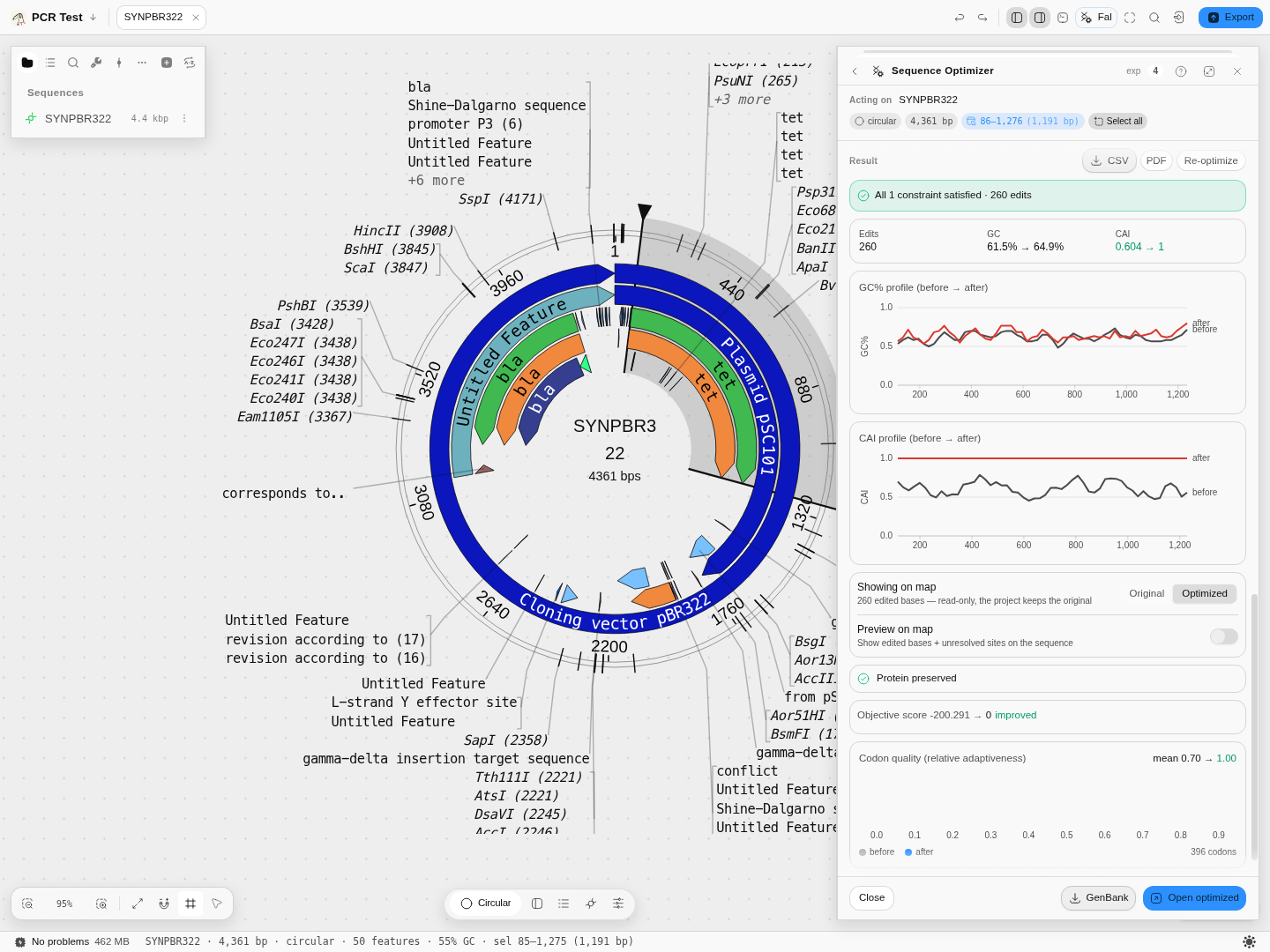 After optimizing
CDS: tet: 260 edits, CAI 0.604 → 1.00, and Showing on map set to
Optimized, so the map, the enzyme labels and the GC readout are all computed from the new bases.
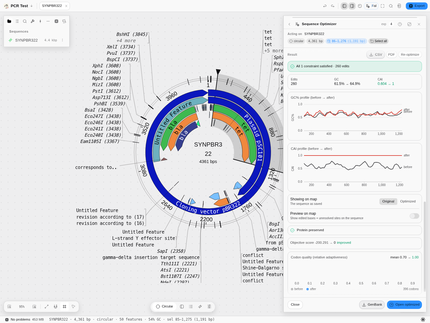 The same run with Showing on map set to Original — the sequence as saved. Comparing the two
is how you find the restriction sites an optimization created or destroyed.
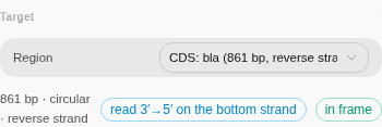 A gene on the bottom strand.
bla in pBR322 is annotated complement(3293..4153), and the panel
says so in two places — because everything downstream, from the codon numbering to the CAI, refers to
the reverse complement of the bases the map is drawing.
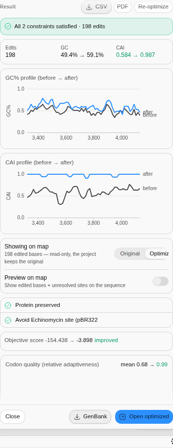 The same gene optimized for E. coli K-12 with the protein protected and a binding-site motif
avoided: 198 edits, CAI 0.584 → 0.987. The profiles are computed along the gene and plotted
against the plasmid's own coordinates, so they line up with the ruler even though the gene runs the
other way.
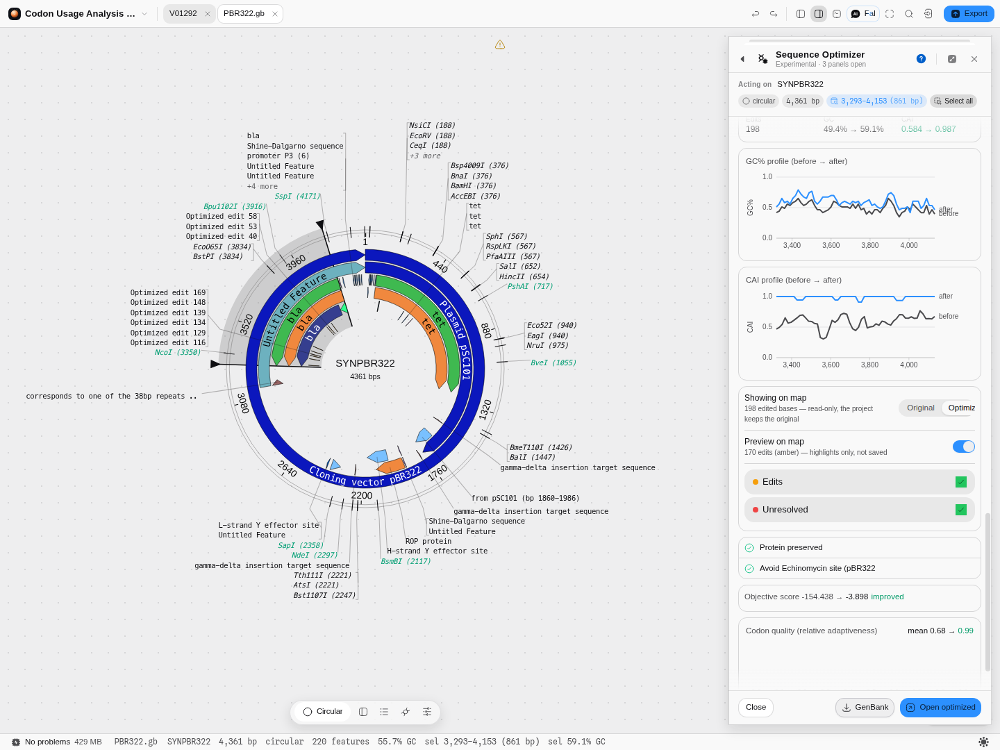 Where the edits landed. Every changed base is drawn on the map inside the gene it belongs to — the
check that a reverse-strand result has been mapped back correctly, and the fastest way to see which
restriction sites an optimization created or destroyed.
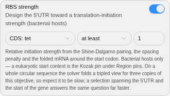 Designing a ribosome-binding site. The anchor names which start codon is being scored, because a
region usually contains more than one gene.
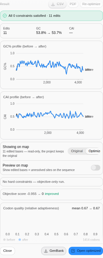 The result of that run on pBR322 — 11 bases changed in the 5′UTR, and the initiation strength lifted
to the floor that was asked for. Nothing else in the plasmid moved.
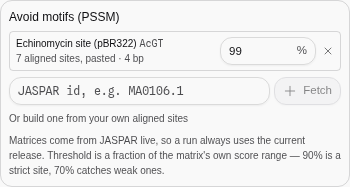 A motif built from sites you paste — here the seven echinomycin-binding sites the pBR322 record
annotates. The threshold is a percentage of the matrix's own score range, so 99% keeps only the
strongest matches.
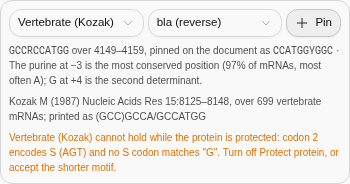 The Kozak context placed around a reverse-strand start codon: the consensus is written into the
plasmid's coordinates as its reverse complement. The last line is the conflict worth knowing about
before you run —
+4 = G needs a second codon beginning with G, and this gene's is serine.

The header states the region the run used, so it still reads CDS: … (1,047 bp) after the canvas
selection has moved on.
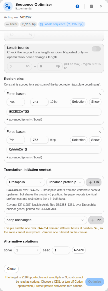
The vertebrate and Drosophila initiation contexts pinned around one start codon. Both pins are kept — the panel names the base where they collide rather than choosing for you.
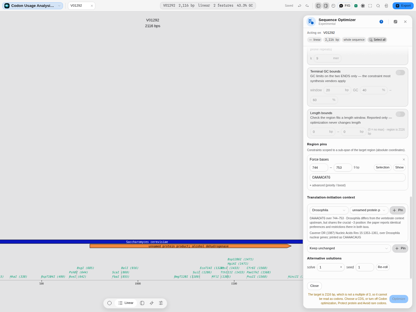 The Drosophila context, which ends at the start codon and so constrains no coding bases: there is
no codon-2 conflict to warn about. The citation under the placement names the string the consensus
is transcribed from, so you can check it against the paper without leaving the panel.
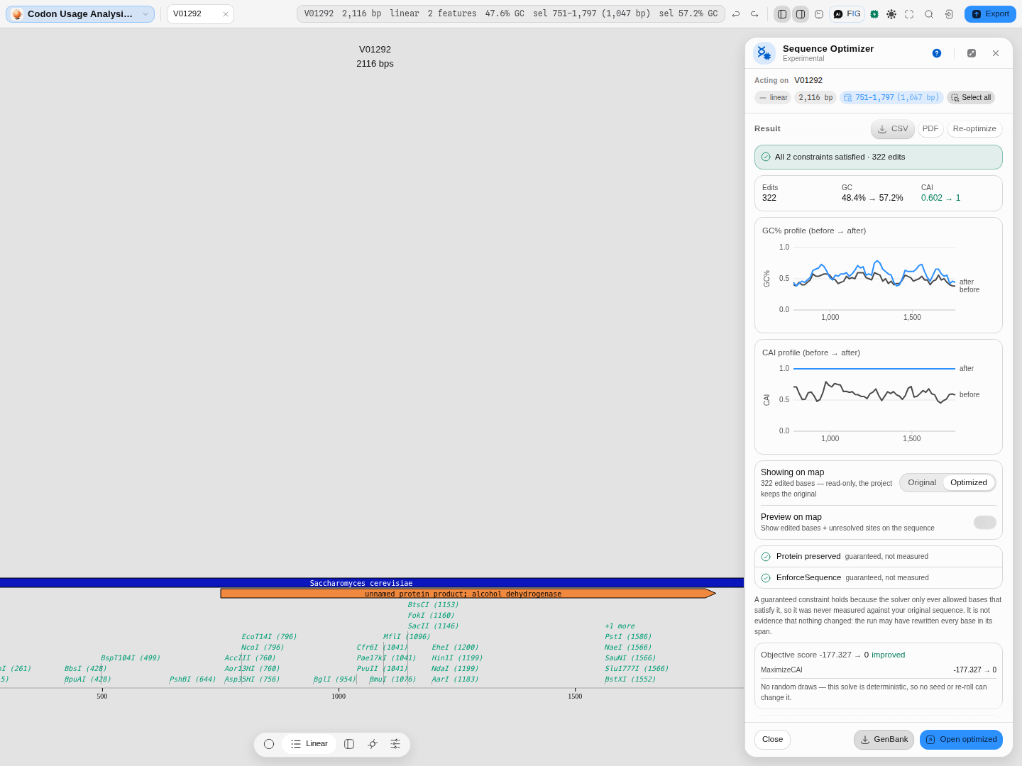 Reading a result. Both constraints here are guaranteed, not measured — the solver enforced them
by construction, so the tick says nothing about the sequence you started with, while the 322 edits
say plenty. Underneath, the objective's own row and the draw count behind the determinism verdict.
Related
In this group: Back-translate: protein → DNA, codon-usage weighted or degenerate · CRISPR Guide Design · Genetic Circuit · In-Situ Probes · CRISPR Edit Inference · RBS & Operon Design · Barcode & Index Design · Auto-Annotate · Apply features from a file · Power and sample size: replicates needed to detect an effect, or the power a design has · Trade-offs: which candidates in a table are not beaten on every objective at once