
Chromatogram
Open a Sanger trace and work on it: inspect the four dye channels, read per-base confidence, correct a base call, trim the noisy ends, and see which positions carry a second peak.
| Reached by | Tools → Sequencing |
| Formats | in: ABIF (.ab1/.abi) SCF ZTR · projects: SeqTrace (.str) · out: FASTA FASTQ GenBank EMBL GCG NEXUS text · projects: SeqTrace (.str) |
| Sample project | Trace samples |
What it does
A Sanger trace is not a sequence. It is four channels of fluorescence sampled a few thousand times along a capillary, plus the instrument's interpretation of those channels — one base call per peak, with a confidence attached. Every question worth asking of a read is a question about the distance between those two things: is this A really an A, is that heterozygous position a real double peak or a dye blob, where does the read stop being trustworthy.
Most viewers show you the picture and the letters and leave you there. This one puts the interpretation under your hands. The base calls are editable, the trim bounds are numbers you can type, the quality track is drawn against the Q20 and Q30 lines you actually cite, and the threshold that decides whether a position is called mixed is a control rather than a constant.
It opens all three container formats a sequencing facility hands out — ABIF from the instrument, SCF and ZTR from the older toolchains — and the same read in different containers gives the same bases. What differs is the metadata, and that difference is visible rather than hidden: see the worked example.
Reading the result, not just the number
Every result on this page states what it found, what would undermine it, and how it was derived. The middle part is the one that changes what you do next, and it is computed from your run rather than written in advance, so it says different things about different reads.
A trim reports the quality it kept against the quality it discarded. Those two numbers are what decide whether the trim did anything: a read whose discarded ends average Q12 against Q34 kept has been cleaned up, and a read whose discarded ends average the same as the ones it kept has been shortened for nothing. The second case is common when a threshold tuned for one instrument meets a read from another, and it is stated rather than left to be noticed. So is the case where less than half the read survives, because everything built on it afterwards is short in proportion.
An ambiguity code in a consensus means two different things, and which one depends on how many reads went in. With a forward and a reverse read, a code is disagreement between them: the two observations of the same base do not match, and the code records that. With ONE read there is nothing to disagree with, and the same code means only that no single base cleared the confidence bar at that position. A high proportion of codes is read the same way: from two reads it points at where they overlap, from one it points at the read itself, and a degraded region will produce codes rather than calls at any bar you choose.
A verification states the fraction of the reference the read actually covered. This is the single most misread number in Sanger verification. One read of 700 good bases against a 2,686 bp plasmid is a clean result over 26% of it, and says nothing whatever about the other 74%. A whole-construct verdict needs reads that span the construct; a clean single read is evidence about the region it spans and no further.
And the other direction is worse, because it reads as a pass. If the reference you picked is SHORTER than the read, the read runs off the end of it and those bases are compared to nothing — so a verification that finds no differences is a statement about however few bases the reference actually holds, not about the read. The coverage figure is bounded by the reference and can never exceed 100%, and a reference shorter than the read is called out by name and by length, with the number of bases that ran past its end, and asks you to check that the reference is the sequence you meant. This is the case a bare no differences would flatter most. Differences are separated by the quality of the base they sit on, because a mismatch on a base below Q20 is more likely a miscall than a change in the clone, and by whether any indels are present, since everything downstream of the first one shifts frame.
A position neither side could call is counted beside the differences, never as one. Where either
the read or the reference carries an IUPAC code compatible with the other base — an N against an
A, an R against a G — nothing disagrees: one of the two sequences simply does not say. Those
positions are reported as uncalled, labelled in the difference table, and kept out of the headline
count and out of the low-quality and codon-consequence readings, because an uncalled base is missing
information rather than a changed one. It is a large correction on real references: a 3 kb M13
reference carrying 14 Ns turns 27 raw disagreements into 8 substitutions, 5 insertions and 14
uncalled over the same alignment, and the 8 is the number that means a difference from the
construct you expected.
A mixed-peak count is a floor set by the threshold you chose, not a total. A second peak is counted when it reaches a set fraction of the primary, so a high threshold admits only near-equal peaks and misses a genuine minor allele below it, while a low one picks up shoulder and dye-blob artefacts alongside real ones. A high mixed rate has two explanations that the count alone cannot separate: two alleles, or a read degraded enough that neighbouring peaks overlap anyway. The read's own mean quality decides which is more likely, and is used to say so.
An absent result says why it is absent. Mixed-peak calling runs on the forward strand, so a track you have reverse-complemented carries no call at all, which is a different fact from a read with no mixed peaks. Both used to look the same; they no longer do.
When you'd use this
Used in: Clone an insert into a vector, and prove it worked · Design a CRISPR guide, check where else it binds, and measure the edit you got
- A read came back and you want to know whether to trust it before you do anything else with it. The status line answers that in one glance — length, mean quality, and the fraction of bases at or above Q20 and Q30.
- You are looking at a specific position — the site you mutated, the junction you cloned, the codon a colleague says is wrong. Jump to it by number, read the peak heights under the call, and override the call if the instrument got it wrong.
- You suspect a heterozygote or a mixed population. Turn the secondary-peak overlay on and set the threshold where you are willing to defend it.
- You are preparing a read for something else — an alignment, a consensus, a submission — and need the noisy ends off first.
To compare a read against a reference and get a list of differences, use Compare Traces to Reference. To grade a whole plate of reads against a construct, use Sequencing Verification.
What this computes
Almost everything here is read off the trace you opened, or computed from its per-base quality. The one exception is stated rather than buried: recomputing quality fits a peak-shape model to the signal, and is described in its own section below.
Per read
-
Phred quality per base, and the read's mean Phred, its ≥ Q20 / ≥ Q30 fractions and the length of its Q20+ stretch
-
The trimmed interval, by either of two methods that answer different questions: Mott's trimming algorithm as the sequencer itself recorded it, or a sliding mean-quality window computed here with the window length and the mean floor as controls.
Autotakes Mott where it exists and says, per track, when it could not — SCF and ZTR carry no instrument trim record -
Secondary (mixed) peaks: the ratio of the second-tallest channel to the tallest at each called base, with the ratio itself as the control, reported as the IUPAC ambiguity code for the two bases involved (
R,Y,K,M…) rather than as a flag, because the code is what a downstream aligner or primer tool understands. Available for ABIF only, and absent rather than zero for SCF and ZTR -
A three-frame translation over the called bases, off until you turn it on, and the per-channel amplitudes behind any base you click
-
Recomputed Phred quality, measured from the trace instead of taken from the file — see Recomputing quality below for what it measures and when the two disagree
-
Bases called from the trace, with their positions and their quality, derived from the peaks rather than read from the file: the count the trace supports against the count the file carries, how many of the shared positions disagree, and the first disagreement as a scan coordinate
-
Heterozygous and mixed base calls, written as the IUB code for the pair (
R,Y,S,W,K,M) at every position the trace supports two alleles, under either of two assumptions about the alleles: equal amounts, which is the diploid heterozygote, or any ratio, for a mixed template, a contaminated read or a pooled sample. Each carries a minimum height ratio as the control, both alleles' Phred values and the four signal measurements behind each, and the alternative calls the search considered and rejected — a position that nearly called heterozygous still leaves its evidence -
A heterozygous insertion or deletion: the breakpoint (as a base and as a scan coordinate) where the read stops being one sequence and becomes two of different length, the size of the indel in bases and in scans, whether the doubling is a genuine indel or a homopolymer stutter and the length of the identical-base run that decided it, and the two allele sequences the doubled trace resolves into. Its diagnostics are reported whether or not one is found: the quality drop measured across the breakpoint against the drop it had to exceed, the number of candidate breakpoints tested, the largest drop seen anywhere in the read, the read's own mean recomputed quality at the finding, and the fraction of the doubled region the deconvolution resolved rather than leaving as
N— the last two being what a positive has to be weighed against, since neither of them is used as a cut-off. A negative therefore carries its own evidence rather than being an empty result -
Base editing quantified from this read alone, with no control trace: for each position of a guide you name, the share of that position's total peak height held by each of the four bases, and a p-value for each against a background model fitted on this trace's own signal outside the guide. What comes back is the percentage matrix over the guide with three bases of flanking context, a bar chart per base with the significance cut-off drawn across it, and the calls that cleared it with their guide position, their position in the read and the change they represent (
C→T,A→G). The model is reported whether or not anything is called — the four fitted zero-adjusted gamma distributions and the cut-off percentage each one implies — because a cut-off nothing in the guide could reach is a different answer from "no editing". The window the background is fitted on is a control, and it is an input to the result rather than a bound on the picture: narrowing it to the clean stretch of the read tightens the noise estimate, lowers the cut-off, and can bring a real signal over it -
Adopting a re-called read, which replaces the read's own base calls with any of these readings so that everything downstream works from them: the sequence you copy or export, the consensus, the verification against a reference and the translation. The signal is untouched — it is the same electropherogram with a second opinion about where the bases are — so reverse-complementing, mixed-peak detection and trimming go on working, and the file's own calls are one click away. Every coordinate already on the read is carried across rather than re-indexed: the trim bounds, each base you corrected by hand and each annotation's ends are matched to the new calls through the scan position of the peak each one sits on, which is the coordinate both callers publish for every base. What that carry could not do is reported rather than absorbed: how many of the previous calls have no peak in the new reading (so anything sitting on one was placed at its nearest neighbour), how many calls are new, any annotation end that had to be inferred from a neighbour, any hand-corrected base the new reading now agrees with, and the furthest a carried coordinate moved, in scans, against the read's own median peak spacing
Across two reads of one template
- A consensus by either of two published methods — Bayesian (the posterior base probability combining both reads' quality scores) or the legacy rule the same tool shipped before it — with a minimum-confidence floor, end-gap trimming and primer trimming as separate stages
- The contig alignment the consensus was actually computed over, drawn column by column, with every position where the two reads disagree marked, so a disagreement is a place to look at both sets of peaks rather than a number in a table
- The count of disagreements, before and after trimming — two numbers, because the difference between them is the part end-degradation explains and the remainder is what you have to adjudicate
Against a reference
- A column-by-column alignment with
|where the read and reference agree and×where they differ, the read's own peaks drawn under each column, and insertion/deletion columns shaded differently from disagreement columns — a gap is a different claim from a mismatch - The differences boxed on the trace itself, once a reference is chosen: every substituted or
inserted call carries a box, a deletion is a bar between the two calls the missing bases fall
between, and a position where one side is an IUPAC code compatible with the other (an
Nin the reference) gets a neutral box, because it is missing information rather than a difference. The count above the read uses the same split as the verification, and hovering a box names the reference base at that position
What it does not compute: it does not phase mixed calls from the trace alone — two heterozygous positions in one read are reported as two IUB codes, and nothing in the signal says which allele at one position travels with which at the next, because the two molecules were sequenced together. Two things here do separate the alleles, and both need something the trace does not contain: Phase alleles splits every ambiguous call into a reference and an alternate sequence against a reference you supply, which resolves the ambiguity rather than the linkage; and the heterozygous-indel reading deconvolves the doubled region into two sequences using the length difference between them. Neither infers a haplotype across independent heterozygous sites. Overriding a base changes the sequence you export, not the peak model, and no quality value is invented for an edited base. Adopting a re-called read does not write a new trace file: the electropherogram you keep is always the one the instrument produced, and an adopted reading is a layer over it that can be removed. Grading many reads against a construct is Sequencing Verification, not this panel.
Where it lives
Tools → Sequencing opens a trace as its own stage tab — a document, not a rail panel — and any
.ab1, .scf or .ztr in the project opens the same way from the file manager. The right rail
edits whatever tab is focused.
A tab holds one or more tracks. That is what makes it part of the editor rather than a viewer: a forward read and its reverse mate sit head to head in one tab, share one zoom and one peak-height scale, and get consensus and batch trimming across both. Each track keeps its own edits and its own undo history, and the rail's (active track) sections act on the one you have focused.
The trace also hands off outward: a read can be opened as a sequence, pushed into the plasmid editor with its annotations, or sent into an alignment with the other tracks in the tab.
Inputs and outputs
In: ABIF (.ab1, .abi), SCF, and ZTR. Nothing else is needed — no index, no reference, no
project setup.
Out: the edited read as FASTA, FASTQ (carrying the per-base quality), GenBank or EMBL (both carrying any annotations you placed) or plain text; a consensus across the tab's tracks; a mutation report when you verify against a reference; and the read itself as a new sequence document or a new project.
What it refuses, and what it says: a file whose bytes are not one of the three trace formats is refused by name rather than opened empty. A read with no per-base quality — which is normal for SCF and ZTR — does not fake one: the quality section says "this trace carries no per-base quality" instead of drawing a flat line at some default, and the controls that depend on quality are disabled with that reason attached.
Demo
Not recorded yet. The screencast worth making is the mixed-peak threshold on
heterozygous.ab1: drag it from 0.33 down to 0.20 and watch three calls become twenty on screen.
Worked example
Open the Trace samples starter. It carries the same read in three containers — forward.ab1,
forward.scf, forward.ztr — plus heterozygous.ab1, a real read with genuine double peaks.
forward.ab1 opens as 730 bases over 10,757 sample points, mean Phred 51.2, with 87% of
bases at or above Q20 and 85% at or above Q30.
Load all three containers as tracks in one tab and press Auto-trim all 3 tracks with the method
on Auto:
forward.ab1                    Mott · 8–641
forward.scf              Win 10/Q20 · 8–655
forward.ztr              Win 10/Q20 · 8–655
That is the whole point of the report being per track. The three files hold the same 730 bases and the same quality values — but ABIF carries the instrument's own trim record and SCF and ZTR do not, so only the first read could be trimmed by the instrument's answer. The other two fell back to the sliding-quality-window scan and stopped 14 bases later. Neither result is wrong; they are answers to slightly different questions, and a single summary line would have hidden that one of your three files was trimmed by a different method.
The ABIF result keeps 634 of 730 bases. The 96 that go are the primer-proximal head and the run-out tail, which is where a Sanger read's errors overwhelmingly live.
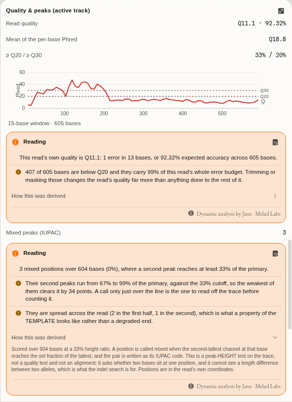
Now open heterozygous.ab1 (605 bases, mean Phred 18.8 — a visibly poorer read) and look at
Mixed peaks (IUPAC) in the quality section. At the default threshold of 0.33 it reports 3
mixed positions: 7 M, 293 K, 582 R. Drag the threshold to 0.20 and the same read
reports 20. Both numbers are real, and the difference between them is the entire scientific
content of the question "is this heterozygous" — which is why the threshold is a control and not a
constant.
The trace samples starter, heterozygous.ab1. The threshold sits at 0.20 — off its 0.33 default,
so the reset affordance has appeared beside it — and the hint below states in words what lowering it
costs you. Both ends of that trade are in the same frame: the control at the top, and at the
bottom Mixed peaks (IUPAC) 20, where the same read reported 3 at the default. The base row under
the trace carries the codes themselves — R, K, S, W, Y — rather than a flag, because the
code is what a downstream aligner or primer tool understands.
Controls
Display
| Control | What changing it does |
|---|---|
| Zoom | Pixels per base, 1–80. Fit width fits the whole read to the viewport; Fit selection fills it with the bases you selected |
| Peak height | Vertical scale of the curves, 0.15–2×. It does not affect base calls — it is how you see a shoulder under a tall neighbour. Fit peak height to the visible window scales to what is on screen rather than to the read's global tallest peak, which is what one dye blob otherwise flattens everything against |
| Colour letters by quality | Base letters take their Phred colour (green ≥Q30, amber ≥Q20, red below) instead of their identity colour. A base with no recorded quality keeps its identity colour rather than reading as poor |
| Confidence numbers | The per-base Phred value above each call |
| Quality track | The confidence bar chart under the trace |
| Dim below | Fades bases under a Phred floor, so the trustworthy stretch stands out. Off/Q10/Q20/Q30 are one click; any value can be typed |
| Auto Y zoom | Re-fits the peak height to whatever is on screen as you scroll, rather than only when the button above is pressed. A Sanger trace loses amplitude along the read, so a scale chosen at base 40 leaves base 700 flat enough to read as a failed run when it is only a scale |
| Show original sequence | A row of the instrument's own base calls under the edited ones, with the columns you changed picked out. It appears only on a read you have actually overridden — with no edits it would be a character-for-character copy of the row above it |
| Translation | Amino-acid lanes under the bases, in the chosen genetic code. Off until you turn it on: of three forward frames, two are noise for a read whose frame you know |
| Frames | All three forward frames, or only the one you are reading. A read whose frame you already know wants one lane; the other two are noise in the height the peaks want |
| Genetic code | Which NCBI translation table the amino-acid lanes are read under. It is not cosmetic: an in-frame TGA is a stop under the Standard code and tryptophan under Vertebrate Mitochondrial, so a mitochondrial read translated under the default shows a premature stop that is not there. All 27 NCBI codes are offered — ids 1–6, 9–16 and 21–33. Ids 7 and 8 were retired by NCBI (merged into 4 and 1) and 17–20 were never issued, so a record naming 7 or 8 predates the merge rather than being corrupt |
| Secondary peaks (mixed) | Draw the second-tallest peak at each position and call it as an IUPAC code |
| Mixed-peak threshold | How tall that second peak must be, as a fraction of the tallest at that base, before the base is called mixed. This decides the answer — see the worked example. Lower it to catch weaker minor alleles and accept more false calls; raise it to keep only unmistakable double peaks |
Base editing
| Control | What changing it does |
|---|---|
| Guide (protospacer) | The 20-base protospacer, 5′→3′, without the PAM. It is matched exactly against this read's own base calls; if it is not there the panel says what it searched for and in which orientation, rather than analysing some other stretch |
| Guide is the reverse complement | Searches for the guide's reverse complement. A C→T edit on the guide strand then reads as G→A in the table, which the reading says |
| p-value cutoff | How improbable a non-reference signal has to be under this trace's own noise before it is called an edit. EditR's own default is 0.01 |
| Guide location | Found matches the guide exactly against this read's own base calls and prints where it landed. Set places it by hand, which is what a read carrying a sequencing error inside the protospacer needs: the analysis then tests the bases you pointed at, and reports a position where the read disagrees with the guide you gave rather than refusing the read |
| Fit the noise on | Auto is the published rule — drop the first 20 bases, then drop every base whose total peak height is under a tenth of the mean of what is left. Manual takes an explicit pair of bounds, which is how the method's authors report a run |
| First base fitted / Last base fitted | The manual window, 1-based and inclusive. Not the read's trim: these bound what the background model is fitted on and leave the read itself alone. Give both or neither. A window that keeps nothing outside the guide is refused, with the guide's own coordinates, rather than answered from an empty fit |
Trim & edits (active track)
| Control | What changing it does |
|---|---|
| History (Undo / Redo) | Steps back through this track's own edits — trim bounds, base overrides, orientation — one at a time. The counts on the buttons are how many steps are available in each direction. This is what you want after an auto-trim you did not like: Reset throws away every edit you have made, undo takes back only the last one. Ctrl/⌘ Z and Ctrl/⌘ ⇧ Z do the same while the trace is focused |
| Auto-trim method | Mott is the instrument's own trim record, present in most ABIF files and in no SCF or ZTR. Window is a sliding mean-quality scan computed here. Auto uses Mott when the file has one and says so when it falls back |
| Window (bases) | How many bases the mean quality is taken over |
| Min mean phred | The mean a window must reach for the read to start, and to keep going at the far end. Raise it to cut more aggressively |
| First base kept / Last base kept | The bounds as numbers, 1-based and inclusive. The two handles on the trace are the same two values |
| Reset trim & edits | Back to the untrimmed read with every base override removed |
Base calls are edited directly on the trace: click a base, type a replacement (IUPAC codes allowed), or arrow along. Edits are per track, undoable, and held separately from the trace data — the curves are never rewritten, so an override can always be taken back. Undo history is per track and starts fresh each time you open the file: edits you saved are restored as the read's state, not as steps you can walk back through.
Navigate
A long read is mostly uninteresting, and the positions worth looking at are scattered through it. These take you to them without scrolling through the rest.
| Control | What it does |
|---|---|
| Next / previous mixed base | Steps the caret to the next position called as an IUPAC code, in either direction. This is how you review a heterozygote: the mixed-peak threshold decides which positions qualify, and these two buttons then walk you through exactly that set. On a read with no mixed calls the control says so rather than doing nothing |
| Go to position | Jumps to a base by number, 1-based, and scrolls it into view |
| Find motif | Locates a subsequence in the called bases and selects it |
| Wrap into rows | Stacks a long read into rows, so the whole trace fits the width instead of running off it. It applies to a single-track read: two tracks are already stacked against each other, and wrapping them too would interleave rows from different reads |
Position and motif are values only you can supply, so the keyboard shortcuts for them open the Navigate section and put the cursor in the field rather than guessing one.
Consensus, Analyze, Verify vs reference and Export are described in their own sections below and on the neighbouring pages.
The five views, and what each one is for
The switcher above the trace changes what the same read is drawn as. All five share one zoom, one peak-height scale and one selection, so moving between them never loses your place.
| View | What you see | Reach for it when |
|---|---|---|
| Trace | The four channels as curves, with the base calls, quality bars and rulers | Reading peak shape — the default, and the only view where a shoulder is visible |
| Split | Peaks above, the base calls as text below, with a divider you can drag | Reading a stretch of sequence while keeping an eye on the peaks under it |
| Sequence | The calls as plain sequence, with quality colouring and translation | Copying, scanning for a motif, or reading a long span quickly |
| Reference | The read's peaks drawn under a reference sequence, one alignment column at a time | Judging a disagreement: is that mismatch real? |
| Contig | Two reads of the same template — a forward and a reverse — stacked at the consensus's columns, with every position where they disagree marked | Merging a pair, and deciding which read to believe where they differ |
Reading a mismatch, not just counting one
A difference table tells you a position disagrees. It cannot tell you why, and the three reasons look identical as letters:
- A clean single peak at the disagreeing position — the read is confident and the template really differs from your reference. This is a variant.
- Two peaks at one position, one roughly half-height — the template is mixed there: a heterozygote, a pooled sample, or an incompletely edited population. The base caller has to pick one letter and will normally pick the taller, so the table shows a plain substitution.
- A smear, a shoulder that migrates, or a run of low peaks — the read has degraded. Nothing about the template is being reported at all, and the mismatches in that stretch are noise. This is typical at both ends of a read and after a homopolymer or a dye blob.
The Reference view is built for exactly that judgement. The reference sits on top, the read's
calls underneath, | where they agree and × where they differ — and the read's own trace is drawn
below, column by column. Mismatching columns are shaded; columns where one side has no base (an
insertion or a deletion) are shaded differently, because a gap is a different claim from a
disagreement.
The alignment is what fixes the columns, not the read's own numbering. That matters as soon as there is one insertion or deletion: from that point on, the read's base 300 is no longer the reference's base 300, and a view that lined the peaks up by read position would show every subsequent base under the wrong reference letter while looking perfectly reasonable. Here the peaks stretch across a deletion and the reference's own numbering stays true.
Click any column to select that base back on the trace, where you can inspect its per-channel amplitudes or correct the call.
Set the reference first. The view is empty until the read has been verified against something — an open sequence tab, a file in the project, or an upload — and it says so rather than drawing an empty frame.
Merging a forward and a reverse read
Sequencing one template from both ends is the oldest quality control in the method, and it works because the two reads fail in different places. A Sanger read is worst at its start (the primer and the dye front) and worst again at its end (the peaks broaden until the caller cannot separate them); the good middle of the forward read covers the bad start of the reverse one, and the reverse read covers the forward's tail. Merge them and you get a contig whose interior is supported twice.
The merge itself is a consensus over an alignment of the two reads, weighted by each base's phred score — the same Bayesian or legacy calculation the Consensus section runs, and the Contig view draws the alignment it actually used rather than computing a second one that could differ from it.
Do this before you look at the contig: reverse-complement the reverse read. The rail's Tracks
section has an RC toggle beside each track, and a reversed track is marked with ↩. Without it
the two reads are being aligned on opposite strands, which produces either no alignment or a
meaningless one, and the view says so rather than drawing something plausible.
Flipping a read you have already worked on is safe. The trim you set, the calls you corrected and the features you drew all move with it: a position becomes its mirror on the other strand, a corrected base becomes its complement, and an annotation flips strand along with its coordinates. So the order does not matter — trim first and flip after, or flip first and trim after, and you end up in the same place. Flipping twice returns you exactly where you started.
The three rows are the whole point. The consensus is on top, then a row per read. Where the two
reads agree the mark between them is |; where they disagree it is × and the whole column is
shaded through both traces. So a disagreement is not a number in a table — it is a place you can
look at both reads' peaks at once and decide which one is telling the truth:
- one clean peak against one messy one → believe the clean read; this is the ordinary case, and it is why the contig is better than either read alone;
- two clean peaks that differ → the template is genuinely mixed at that position, or the two reads came from different molecules;
- both messy → the contig has no real coverage there, whatever the consensus letter says.
Step by step, on the bundled sample. Open the Trace samples starter, which ships a real forward/reverse pair of one earthworm COI barcode amplicon:
- Open
Achl_ACHLO006-09_1_F.ab1from the file list. It is 703 bp, mean Q55. - In the rail's Tracks section press + Add track (fwd/rev) and pick
Achl_ACHLO006-09_2_R.ab1(705 bp). The tab now holds two tracks. - Press RC beside the reverse track. It gains a
↩. - Switch the canvas to Contig. You get a 746 bp consensus over 662 columns covered by both reads, with 31 disagreements — the count is in the strip along the bottom.
- Look at where the shaded columns are: nearly all of them sit in the first and last tenth of the contig, which is exactly where both reads are worst.
- Now trim. Auto-trim every trace in the All open traces section runs the quality trim over every open tab at once. The contig becomes 717 bp over 656 shared columns with 25 disagreements.
That last step is worth dwelling on, because it is the opposite of the tidy result you might expect: trimming removed six of the thirty-one, not most of them. End-trimming takes away the disagreements caused by degradation; the ones that remain are in the good part of the read and are real disagreements between the two molecules. A trimmed contig is cleaner, not finished — those 25 positions are the ones you actually have to adjudicate, and the Contig view is where you do it.
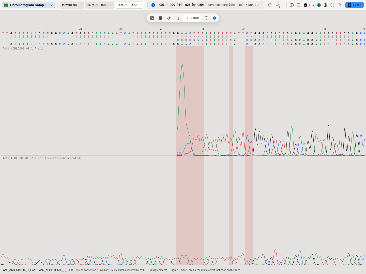
Fitting the width fits the CONTIG. Press Fit width on this view and it fits the consensus's 746 columns, not either read's 703 or 705 bases — an alignment is longer than the things aligned, and a fit that used a read's length would leave the last few dozen columns off the edge.
The two bands share one peak height, and each is drawn against its OWN read's tallest peak. That is what makes them comparable by eye — the same vertical scale means the same thing in both bands — but it also means one read's 5′ dye blob can flatten the rest of that read while the other band looks normal, which is what the picture above shows. Fit peak height rescales to the peaks in the window you are looking at rather than to the whole read, and on this view it fits the active read and says which one it used, because one number cannot be right for both at once. If a band reads as a dead run, scroll to it and fit before believing it.
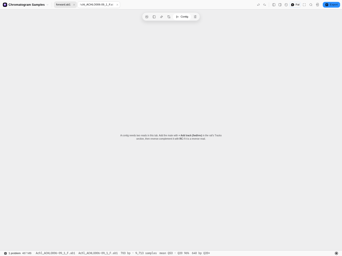
One read in the tab? The view says so and names the control that fixes it, rather than drawing an empty frame:
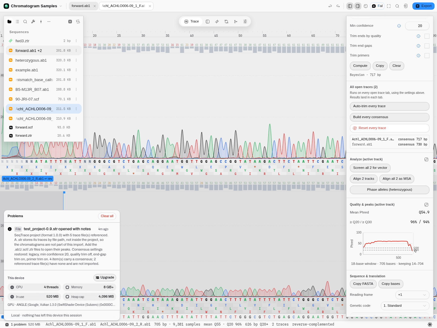
SeqTrace projects (.str), in and out
If you have older Sanger work in SeqTrace, its .str project files open here directly: drop one
in and you get the consensus sequence of every item the project had analysed, its notes, and the
forward/reverse pairing it recorded, together with the consensus settings it was using (algorithm,
minimum confidence, and which of the three trimming stages were on).
What does not come back is the chromatograms, and this is a property of the format rather than a
limitation here: a .str refers to its trace files by their path on the machine that saved the
project, so the peaks live in the .ab1/.scf/.ztr files beside it and not inside the project.
The import says exactly that, and names how many trace files the project referenced, so you know
what to go and find. Add those files to the project and their peaks open normally.
Items the project never analysed contribute nothing — an item with no saved consensus is counted in the import's note rather than opened as an empty sequence.
Writing one back out
The round trip closes: Export ▸ SeqTrace project (.str) writes every open trace tab back into a project file SeqTrace itself will open. Its scope is the whole set of open reads, not the one in front of you, and what it records is exactly what the format holds:
- The consensus settings — algorithm, minimum confidence, and the three trimming stages with
their windows and primers. A
.strcarries one settings block for the whole project, and so does the panel, so there is nothing to reconcile between the two. - Each read's consensus, where you built one, together with its notes.
- The forward/reverse pairing. A tab holding two reads is written as the paired item SeqTrace stores a fwd/rev contig as, with the two reads as its members and the reverse one marked.
- Not the chromatograms — the same property that limits the import limits the export. The file names the reads and the peaks stay in the trace files, so send those alongside it.
A read you have edited exports as you have it: trimmed bounds applied, base overrides included.
Two practical notes. A tab holding more than two reads is written as the pair plus the extra reads as their own items, because a paired item holds exactly two members in the format and inventing a third would produce a file SeqTrace declines to open. And an unanalysed read is written as an unanalysed item, exactly as SeqTrace writes one, rather than being dropped.
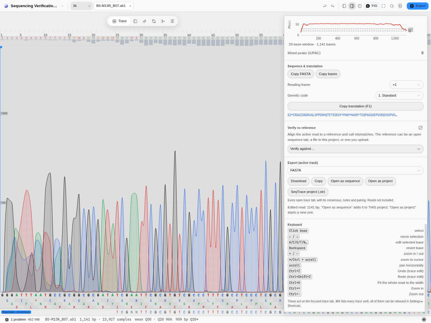
A read with its Bayesian consensus built (the consensus row sits under the trace), and the export
that writes it, its settings and its notes back into a .str.
Running something over every open read at once
The rail's All open traces section appears once you have more than one trace tab open, and runs three things across every one of them: Auto-trim every trace, Build every consensus and Reset every trace. Each reports per tab rather than as one number, because the answer genuinely differs between reads — an ABIF file usually carries the instrument's own trim record and an SCF or ZTR file never does, so two tabs trimmed in the same click can be trimmed by two different algorithms, and you are told which.
Each result lands in the tab it belongs to: the consensus built for a tab appears in that tab's own Consensus section, so there is one place a consensus lives whether you built it for one read or for twenty.
Algorithms you can choose
Trimming — two methods, and they answer different questions.
- Mott's trimming algorithm, as recorded by the sequencer itself. The instrument computes a running score from the base qualities and stores the highest-scoring stretch in the file. Reach for it when you want the same answer your facility's own software would give, because it is literally that answer read back out.
- A sliding mean-quality window, computed here from the per-base Phred values, with the window length and the mean floor as controls. Reach for it when the file has no Mott record (every SCF and ZTR), when you want the same rule applied to a mixed set of files, or when you disagree with the instrument.
- Auto takes Mott where it exists. It is the default because agreeing with the instrument is the better default; it tells you, per track, when it could not.
Base editing — asking a different question from ICE and TIDE.
A nuclease makes a double-strand break, the cell repairs it badly, and what you are left with is a pool of insertions and deletions. That is what ICE and TIDE decompose, and both of them need a control trace from unedited cells to decompose against. A base editor makes no break and no indel: it converts one base to another inside the protospacer, and the only evidence in the trace is a second peak under the called base. Both indel methods are blind to it, and no control trace is required to see it.
The method here is EditR (Kluesner et al., The CRISPR Journal 1(3)
–250, 2018). It works from one read:- Every called base is expressed as the share of that position's total peak height held by each of the four channels.
- The positions outside the guide are taken as the background: at a base that is not edited, a non-reference channel is reading noise. Each of the four bases gets its own zero-adjusted gamma fitted to its own noise, because the channels are not equally noisy.
- Each position inside the guide is then asked how improbable its non-reference signal would be under that base's own noise model, and called when it clears the p-value cut-off.
The window the background is fitted on is an input to the answer. This is the part worth
understanding before you trust a single call. The published rule drops the first 20 bases and then
every base whose total peak height is under a tenth of the mean of the rest, which is a reasonable
automatic choice and not the only one. Narrow the window to the read's clean stretch and the noise
estimate tightens, the cut-off drops, and a signal that sat just under it moves above it. The
bundled PD-1_cytosine_base_edit.ab1 is the case to run: with the window left automatic it returns
the two positions the method's authors publish — a 40.9% C→T at guide position 8, the signature of a
cytosine base editor, and an 8.2% G→A at position 5 that the same authors label a false positive.
Set the window to the authors' own 20–433 and a third position appears, at guide position 14 and
6.3%. Nothing about that signal changed. The cut-off moved.
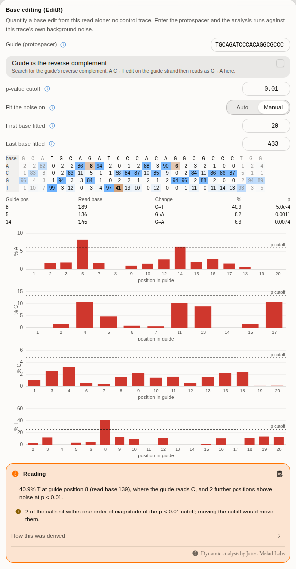
The percentage matrix over the guide with three flanking columns of context, one bar chart per base with the cut-off drawn across it, and the three calls the tightened window produces. Every cell of the matrix jumps the trace to the base it describes.
Which is why the section reports percentages and p-values rather than a count of hits. Two of those three calls are at the noise floor and one is a real edit at 40.9%; a surface that answered "three positions edited" would be telling the truth and communicating something false. The reading under the result says how many calls sit within an order of magnitude of the cut-off, because those are the ones a different window would move.
When the guide is not found. The search is an exact match, so one sequencing error inside the
protospacer is enough to miss it, and the panel says what it searched for and in which orientation
rather than analysing some other stretch. Switch Guide location to Set and give the bases to
test: on the bundled read, a guide with a single substitution at its first position is refused,
placed by hand at 132–151 it returns the same two published calls, and it reports a 98.9% difference
at the position where the read disagrees with the guide you gave. That is the honest answer to "test
these bases", not a failure.
What it cannot tell you. EditR's premise is that the signal outside the guide is clean. After a nuclease cut the whole 3′ tail is a mixture, the background absorbs it, and the test cannot fire at all — on such a read the section says so and points at ICE and TIDE rather than reporting a negative that was never possible. It also needs a re-derived peak matrix, which means an ABIF with the instrument's edited base-call tags: SCF and ZTR reads cannot be analysed this way, and the panel says that rather than showing an empty table. One diagnostic upstream computes is deliberately absent and named as absent: the Filliben goodness-of-fit coefficient, which is read off randomised quantile residuals and so depends on a random-number stream rather than a formula. It enters no percentage, no p-value and no call.
Recomputing quality — measuring confidence instead of reading it.
The Phred values in a trace file are the instrument's opinion, produced by its own basecaller under its own calibration. Recompute quality from the trace measures four properties of the signal at each called base and looks the resulting combination up in a table calibrated against reads whose true sequence was known. The four are the entire input, so a score is never a bare number:
- Peak height ratio, over a window of three called peaks and again over seven: the tallest uncalled peak in the window divided by the shortest called one. A high value means something that was not called is nearly as tall as something that was, which is the shape of a mixed position or a mis-call.
- Peak spacing ratio, over seven called peaks: the widest gap between consecutive peaks divided by the narrowest. Peaks march evenly while a read is healthy and stop doing so as it degrades.
- Peak resolution: how far the fitted peak-shape model sits from the data at that base.
The calibration table is a choice you make, not a default applied on your behalf, because the tables are specific to an instrument and polymer: the same signal scores differently under ABI 3730 Pop-7 than under ABI 3700 Pop-5, and a confidence figure is not interpretable without knowing which one produced it.
Expect the two scales to disagree, and read the disagreement rather than averaging it. On a typical read most bases change, because the instrument and this table were calibrated on different material. The recomputed values are useful when you want every read on one footing — comparing runs from different machines, or re-scoring an archive whose original calibration you no longer know — and the instrument's own values are the right ones to quote when you are reporting what your facility's pipeline produced.
Calling the bases from the trace. The same measurement supports the stronger question: not how good is this call, but what does the trace actually say here. Under Measure you can switch from re-scoring the existing calls to calling the bases from the trace, which discards the instrument's calls and derives the bases, their positions and their quality from the peaks themselves.
A re-called read can be a different length from the file's. The caller inserts bases where the peak spacing says one was missed and drops calls the peaks do not support, so a read the instrument wrote as 730 bases can come back as 701. The panel therefore reports both counts, how many of the shared positions disagree, and the first disagreement as a scan coordinate you can click to land on that peak, so the first thing you do with a disagreement is look at the signal that caused it.
When the two disagree, neither is automatically right, and the peak is the evidence. The instrument's calls are what your facility's pipeline reported and are the ones to quote as such; the re-called sequence is what the trace supports independently of the instrument's own basecaller, which is what you want when the original calibration is unknown or the read is being re-examined after the fact.
Calling two alleles at once. A third and fourth reading ask something the first two cannot: at
every called position, is there a second base under the first? Call heterozygotes and Call
mixed bases derive the calls from the peaks exactly as above, and additionally score each position
against the alternatives the trace supports, writing the two-base IUB code (R, Y, S, W, K,
M) where a pair wins.
The two differ in one assumption, and it is not a matter of strictness:
- Heterozygotes assumes the two alleles are present in equal amounts, which is what a diploid heterozygote produces, and scores each allele at half the pair's height.
- Mixed bases assumes nothing about the ratio, and scores each allele at its own share of the pair's height. That is the reading for a mixed template, a contaminated read, or a pool.
They genuinely disagree: across this tool's own validation corpus of 5,605 called bases, the two differ on 348 calls and on 698 quality values. Choosing between them is choosing what you believe about the sample, so neither is offered as the default reading of the other.
A mixed call scores lower than either of its halves, and that is not a defect. The call is right only if both alleles are right, so the two accuracies multiply: a pair of Q30 alleles is a Q27 call. The panel shows each allele's own Phred value and the four signal measurements behind it beside the pair's, so the number is always traceable to the two peaks that produced it.
The minimum height ratio is the control: how tall a second peak must be, as a fraction of the called peak, before the search considers it as an allele at all. Lowering it widens what is considered — the number of alternatives kept rises steeply — but that is not the same as calling more mixed bases, because a rejected competitor can change which call wins at a position. The default is the published one, 0.1.
Every position the search scored and did not call is kept as an alternative, with its own quality value. A heterozygous position the thresholds turned down is therefore visible rather than absent, which is the difference between "there is nothing here" and "there is something here that did not clear the bar".
A heterozygous indel is a different question, and neither reading above can answer it. Both ask, at one position, whether two bases are present. A heterozygote carrying an insertion or a deletion on one chromosome produces something else entirely: the read is clean up to the indel and then a superposition of two sequences offset by the indel's length, all the way to the end. Every position after the breakpoint carries two peaks, so a per-position test reports a wall of ambiguity codes and never names the cause.
Detect a heterozygous indel asks the question directly, in three steps:
- Where does it start? It walks the read for the first position where the second peak stops being noise, where the doubling stays self-consistent under a shift of a whole number of bases, and where the quality values drop — a real breakpoint degrades every call after it. A homopolymer run that merely stutters is separated from a genuine indel by the length of the identical-base run behind it.
- How long is it? The four dye channels after the breakpoint are autocorrelated. A signal that is two copies of itself offset by k scan points peaks at lag k, so the lag of the tallest secondary peak is the indel's length. Divided by the run's scans-per-base, that is the length in bases.
- What are the two sequences? At each position after the breakpoint there are two candidate
peaks and two alleles to assign them to. Each is assigned by asking which reading stays
consistent with the peak one indel-length away — forwards for the short allele, backwards for the
long one. Positions where neither assignment is forced are left as
N, in both alleles. That is not a low-quality call; it is the trace declining to decide, and filling it in would be a guess presented as a read.
The quality drop is the gate, and it is reported whether or not an indel is found: a read that carries none says so with the largest jump it measured, against the value it had to exceed, and with the number of breakpoints it tested to get there. Those are two different negatives and the panel distinguishes them, because they mean different things: no position doubled convincingly enough to be tested is a statement about the trace, while positions doubled and none of them showed the quality drop is a statement about the evidence at those positions.
How well it works, measured against reads whose answer is known. Agreement with a reference implementation is not accuracy, so the detector was run over three labelled sets from three laboratories — matched pairs where each control is a read of the same region without the indel, so the answer follows from how the read was made rather than from what a program says about it. Two of the sets are CRISPR editing experiments; the third is a pair of siblings, one carrying a small heterozygous indel and one not, and that pair is one you can open here — it is in the Trace samples. Seventeen reads, seven of them carrying a length-changing difference:
- 7 of 7 detected. Every read with a real insertion or deletion in it was found, including the sibling pair you can open and check yourself.
- The same read in two file formats gives the same answer — one of the seven ships as both an ABI and an SCF, and the breakpoint, the size and the two alleles come back identical. Worth knowing because two tabs holding "the same" read disagreeing is the failure this rules out.
- The size is right, and it was checked against a different method. One of the seven is independently quantified rather than merely labelled: its own publication decomposes it as a one-base deletion, and the search reports a one-base deletion. That is a second measurement of the same quantity by a different technique, which agreement with a reference program cannot supply.
- It found that deletion at roughly 23% of the template, not at the clean 50/50 of a textbook heterozygote — the second sequence is about a third the height of the first and is still resolved. Take ~23% as the lowest fraction demonstrated here, not as a claim that any fraction works.
- Silent on the substitution-only edit. One pair in the set is a homology-directed repair donor that changes bases without changing length — an edited read with no indel in it. It is reported as carrying none, which is the case that separates "finds edits" from "finds indels". A detector tuned until it fired here would have been worse, not better.
- Silent on 9 of 10 known negatives, among them the matched sibling of one of the positives — the same region in the same family without the indel, which is the sharpest control available. On that one and on the cleanest CRISPR control it reaches zero candidate breakpoints rather than testing some and rejecting them: the stronger of the two negatives, and the panel says which one you have.
- 1 of 10 known negatives fired, on the deliberately degraded read: an unedited amplicon with poor signal, mean recomputed quality Q19.1. This is the algorithm behaving as its physics implies — as a read degrades, the second peak stops looking like noise, and the quality decline that gates the test is present for the same reason the read is decaying.
No quality cut-off is applied to suppress that false positive, and the reason is stated because it
is the more useful fact. The obvious fix is to refuse to answer below some mean quality. It does
not work here: the false positive sits at Q19.1 and a genuine edit in the same set sits at
Q19.5. The second candidate discriminator — how much of the doubled region the deconvolution
resolves rather than leaving as N — does not separate them either, at 81.6% against 88.1%. Fitting
a threshold to a handful of points would produce a number that looks like it works and was never
measured, so the panel reports both figures beside the result and says what they do and do not tell
you instead.
What that means when you use it. A positive on a clean read is strong: no clean read in any of the three labelled sets produced a false one. A positive on a degraded read is a reason to look at the trace, not a result — the panel names the read's own mean recomputed quality next to the finding so you can see which situation you are in. A negative carries the number it failed on, so it can be argued with.
There is one choice of reading here that other tools do not offer, and it is stated rather than hidden. The reference implementation this is validated against contains a defect in how it reads its own quality values: it measures a quality drop of zero at every base of every read, so its indel detector cannot fire on any trace at all. Both readings ship, both are validated against a build of the reference program that performs them, and the corrected one — the reading the reference implementation's own interface declares — is the default, because it is the only one that can answer the question. The other is kept so a result can be reproduced against the published program exactly.
All five modes are reachable four ways — the trace panel, the command palette, the canvas menu and the trace's own right-click menu — and the assistant you can talk to in the editor is told when you have run one, including which calibration table it was scored on.
Every reading is also available by asking, not only by clicking: the assistant can re-score a read, call its bases from the trace, call its heterozygous and mixed positions, or search it for a heterozygous indel — on the read you have open or on one named by file, scored against whichever calibration table you name and, for the mixed readings, at whichever minimum height ratio you name. It runs the same measurement the panel runs and reports the table, the mode and the ratio it used, so the two cannot disagree. The indel search is also a pipeline step, so a batch of reads can be gated on whether each carries one, and either allele carried onward as a sequence.
If you agree with the re-called read you can take it: Open as sequence puts it in the project as an ordinary sequence, carrying a whole-length annotation recording that it was called from the trace rather than read from the file, so it cannot later be mistaken for the instrument's own; Download FASTQ writes it out with the recomputed quality alongside it. It does not overwrite the read on screen — a re-called read is usually a different length from the file's, and the two are worth keeping side by side.
Consensus — two published methods.
- Bayesian (the default): the posterior base probability at each position, combining both reads' quality scores, so a high-quality call on one read outweighs a poor conflicting call on the other.
- Legacy: the older rule the same tool shipped before the Bayesian model.
They agree far more often than they differ, and where they differ it is at exactly the low-quality
positions you should be looking at anyway. On forward.ab1 alone the two produce the same 730-base
consensus with the same 96 N calls at the default minimum confidence of 20.
Mixed-peak calling has one method — the ratio of the second peak to the first — and the ratio itself is the control. There is no second opinion to offer here; the disagreement in the field is about where to put the threshold, not about how to measure it.
Bring your own: the Python and R consoles mount the project's files, so your own trace-handling
code runs over the same .ab1 in the same browser tab.
The science
Phred quality is the scale everything here is measured on: Q = -10 log₁₀ P(error), so Q20 is
one wrong base in a hundred and Q30 is one in a thousand. That is why the quality track draws rules
at 20 and 30 rather than at round fractions of the axis, and why Dim below offers those two as
presets — they are the thresholds papers actually quote.
Mott's algorithm is the trimming rule the sequencer applies: convert each base's quality into an error probability, subtract a cutoff, and take the contiguous stretch whose cumulative score is highest. It is the standard because it finds the best interval rather than nibbling from each end independently, so a single bad base in the middle of a good read does not truncate it.
The consensus builder is the one from SeqTrace, both of its methods, including its end-gap and primer trimming stages. The Contig view draws the alignment that same builder used to produce the consensus above it, rather than aligning the two reads a second time — so the peaks you are comparing at a disagreement are in the columns the consensus was actually computed over.
Secondary peaks are found by re-deriving the peak window at each called base and measuring the
next-tallest channel within it. A base is called mixed when that second peak clears the threshold,
and it is reported as the IUPAC code for the two bases involved — R for A/G, Y for C/T, K for
G/T, M for A/C, and so on. Reporting the code rather than a flag matters: the code is what
downstream alignment and primer tools understand.
On correctness: the trace readers, the trimming, the consensus and the secondary-peak detection are checked against the reference implementations they come from — SeqTrace for consensus and trimming behaviour, and the trace-format readers against the same corpora those libraries test on — byte for byte, on every release.
Shared with other tools: Read quality compares how every tool that does this chooses its method.
Limitations
- SCF and ZTR carry no instrument trim record. Asking for Mott on one falls back to the sliding window. This is stated in the outcome line rather than silently substituted, but it means "the same read" can trim differently depending on which container you were sent.
- The mixed-peak threshold has no universally correct value. 0.33 is the default because it is the one the detection was published and compared against, not because it is right for your chemistry. A read with a strong dye blob will produce false mixed calls at any low threshold.
- Secondary-peak detection needs the raw ABIF trace. It is unavailable for SCF and ZTR, and the overlay and its threshold do not appear for those files rather than reporting zero — zero would be a claim, and absence is the truth.
- Heterozygous-indel detection loses specificity on a degrading read. Across three labelled sets it found 7 of 7 real indels and stayed silent on 9 of 10 negatives, with its one false alarm on the poorest-signal read of the seventeen. No quality floor is imposed to hide that, because the measured qualities of the false positive and of a true positive are Q19.1 and Q19.5 and do not separate; the read's own quality is reported beside the finding so the judgement is yours and is informed.
- Only the first heterozygous indel in a read is reported. The method depends on everything after the breakpoint being two copies of one sequence offset by one length. A second indel further along breaks that assumption rather than appearing as a second result.
- The two deconvolved alleles are not a second read of the sample. Positions where neither
assignment is forced come back as
Nin both alleles, and the fraction resolved is reported for exactly that reason — an allele that is 20%Nis a hypothesis to check against a fresh read, not a sequence to deposit. - Mixed calls are not phased. Knowing that positions 7, 293 and 582 are each heterozygous does not tell you which variants travel together; allele phasing across a read is a separate operation and only resolves the simplest cases.
- Base-call edits do not re-call the trace. Overriding a base changes the sequence you export, not the underlying peak model, and no quality value is invented for an edited base.
- This is one read at a time. Grading many reads against a construct, or screening a plate, is Sequencing Verification — not this page.
Compared with other tools
Sourced from each vendor's own pages, retrieved 2026-08-08.
SnapGene imports .ab1 traces, aligns them to a reference and assembles Sanger contigs. Its
Sanger workflow is more opinionated than this one and its alignment-to-reference view is mature;
what it does not offer is a threshold you can move on the mixed-peak call.
Geneious Prime covers Sanger trace editing within a much wider sequencing suite, including read mapping and de novo assembly, which this workbench does not do at all.
What is different here rather than better: every parameter that changes a number on screen is a control with its range and its default stated, the file opens in a browser tab with nothing installed and nothing uploaded, and the same read in three containers can be opened side by side to see where the containers disagree. What is genuinely missing compared with a full suite: contig assembly across many reads, and any of the upstream NGS work.
Export
- FASTA — the edited, trimmed read.
- FASTQ — the same bases with the instrument's per-base quality, Phred+33. This is the only format here that keeps the confidence, so it is the one to reach for when the read is going on to anything that weights bases by how well they resolved: an assembler, a variant caller, a QC report. One quality value per base, always in step with the bases beside it, because both come from the same trimmed window.
- GenBank — with any features you annotated on the read.
- EMBL — the same record in EMBL's flat-file form, feature table included. GenBank and EMBL are written from one record, so a feature that reaches one reaches the other: the choice is which convention the tool you are handing it to expects, not which annotations survive.
- GCG — single-sequence GCG with its checksum.
- NEXUS — a data block, for phylogenetics tools.
- Text / Line — the bases alone, wrapped or on one line.
- Download all n — every track in the tab in one go.
- SeqTrace project (
.str) — every open trace tab as a SeqTrace project: settings, each consensus, notes and pairing. Described in full under Opening a SeqTrace project. - Open as sequence / Open as project — the read becomes an editable sequence document or a new project, rather than a file you saved and re-imported.
- Download SeqTrace project (
.str) — every open trace tab in one project file (below).
Exports are of the read as you have it: trimmed bounds applied, base overrides included.
What each format DROPS, said before you write it. A sequence file that is missing something opens perfectly well somewhere else; nothing downstream will tell you the annotations or the quality were never in it. So the panel states, for the export you are about to make, what this target does not carry — the per-base quality on anything but FASTQ, the annotations on anything but GenBank and EMBL, and the bases a trim has removed — together with how many of each this particular read stands to lose. A read with no annotations loses nothing by going out as FASTA, and it says that too rather than warning you about a loss you were never going to take.
What the read is called. A trace carries two names and they often disagree: the file name it
reached you as, and the sample name the sequencer itself recorded (SMPL in an ABIF, NAME= in an
SCF or ZTR) — usually the plate well or the sample id the run sheet used. Name picks which one
the record header, the LOCUS line and the downloaded file carry. On the bundled reads the two really
do differ: forward.ab1 was run as O1. Where a file records no sample name, the file name is used
and the choice is disabled rather than blanking the header.
Extension. .fa and .fasta are the same bytes, and so are .gb and .gbk; which one is
right depends on what you are handing the file to. Each format's suffix is yours to set, and the
filename the download will carry is shown under it.
One thing worth knowing about quality on a base you edited. If you override a call, the FASTQ still carries the confidence the instrument measured at that position. That is deliberate: a Phred score describes how cleanly the peak resolved, which does not change because you read the peak differently. It is not an endorsement of your call, and it is not a claim that the position was re-measured. If you want the distinction recorded, annotate the base — annotations travel in the GenBank export.
Your consensus parameters are part of the project, not of the session: change the minimum confidence or turn a trimming stage on, and it is still set that way when you reopen the project tomorrow.
API
There is no separate scripting entry point for the trace panel beyond the consoles described under Algorithms. The Python and R consoles mount the project's files, which is the supported way to run your own analysis over the same trace.
Automation
Trimming and writing a read out are both pipeline steps. Trim a Sanger read takes a read and either of the two trimming methods and reports the interval it kept; Export a trace takes a read, one of the eight formats, and optionally a trim, and hands back the file as text. Chained, they are the "trim these forty reads and export FASTQ" job that used to have to be done a tab at a time. Both steps offer the same choices as the panel and open on the same defaults, so a pipeline cannot quietly trim to a threshold nobody picked or write a format the panel would not have written.
Both are reachable the same three ways everything here is: the panel, a step in a workflow, or by asking the assistant for it.
What is still done in the tab. Building a consensus over a plate, and the per-read editing the panel exists for — an override, an annotation, a trim you place by eye. The batch operations inside one tab (auto-trim all tracks, reset all, download all) remain the way to act on the reads stacked in front of you.
Provenance
Every document edit — a base override, a trim, a reverse-complement, an annotation — is a step in the tab's own undo history, held per track and separately from the trace data, so the original curves are always recoverable.
Citing a number from this page means citing the method, not the tool: Mott's algorithm for a trim bound, Phred for a quality figure, SeqTrace's builder for a consensus, and — for a mixed-peak count — the threshold you used, because the count is meaningless without it. A recomputed quality value carries one more thing: the calibration table it was scored against, which the panel names beside the result. Both the recomputation and the calling from the trace are checked against TraceTuner, base for base, on every read in the bundled sample set — every base, every position and every quality value, with nothing sampled.
The heterozygous-indel search is checked twice over, because agreement and accuracy are different claims. It is graded against TraceTuner for agreement — the breakpoint, the size, the stutter test, the quality jump and both deconvolved allele sequences, exact, on every read in the sample set and at forty additional breakpoints supplied by hand — and separately against three labelled sets from three laboratories, where the answer comes from how each read was made rather than from any program: 7 of 7 length-changing differences found, one of them with its size confirmed against an independent published decomposition of the same read, silence on a substitution-only edit and on a matched sibling control, and one false positive on the degraded read, reported above rather than tuned away. Citing a positive means citing the read's mean recomputed quality with it.
The base-editing percentages and p-values are checked against the method's own published implementation — every position of the guide and every base, no sampling, with the four fitted noise models and the four cut-off lines graded alongside them — and separately against what its authors publish in prose for the read bundled here: the edited position, its percentage, and the position they themselves label a false positive. Citing a call means citing three things with it: the p-value cut-off, the window the background was fitted on, and the percentage, because the first two are what decided that the third cleared the line.
What an export carries, and what it cannot. A read can leave as plain bases (FASTA, GCG, NEXUS, GenBank, or as text), or as FASTQ, which is the only one of them that also carries the per-base quality. None of them carries the trace: the four channels, the peak positions and the instrument's own metadata are not written back out, because writing a chromatogram file is not something this tool does. Nothing is lost by exporting — the file you opened is never rewritten, and your edits are kept beside it — but an export is a projection of the read, not a copy of the chromatogram. If you need the chromatogram itself, keep the original file.
Screenshots
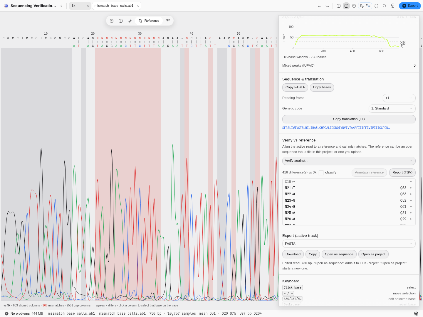
The Reference view. A 730-base read against a 3 049-base M13 reference: 603 columns aligned,
166 of them mismatching. The long shaded block on the left is the run of N calls at the read's 5′
start — the region where the peaks below show why the caller refused to commit, which is the whole
argument for looking at the trace rather than the table.
Above. The trim section of the same rail, with three containers of one read trimmed by two different methods, is captured in the worked example's report.
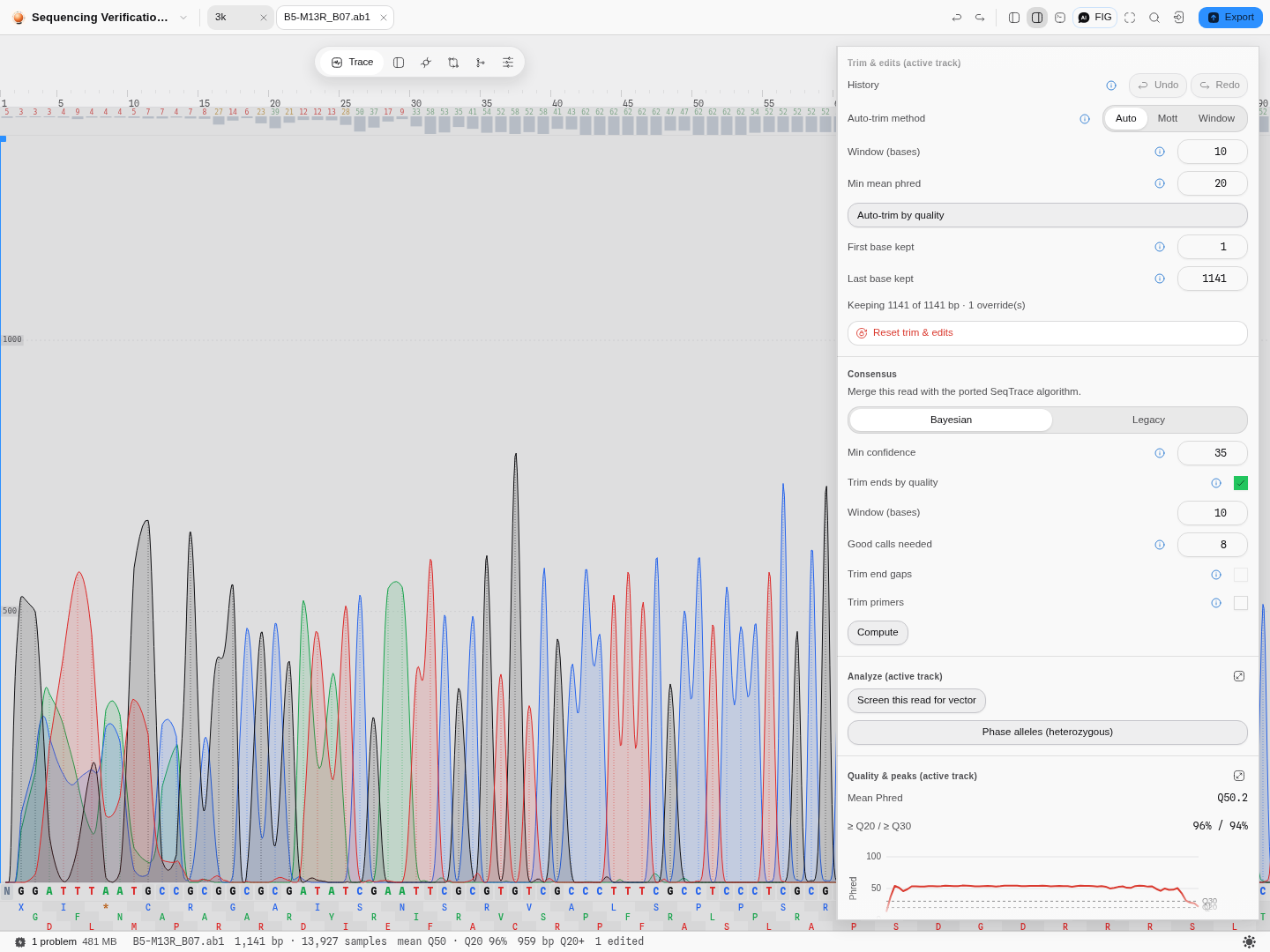
Your parameters are project state. Minimum confidence at 35 with end trimming on, a hand-edited
base showing as N on the canvas and counted as one override in the trim section — all of it after
closing and reopening the project.
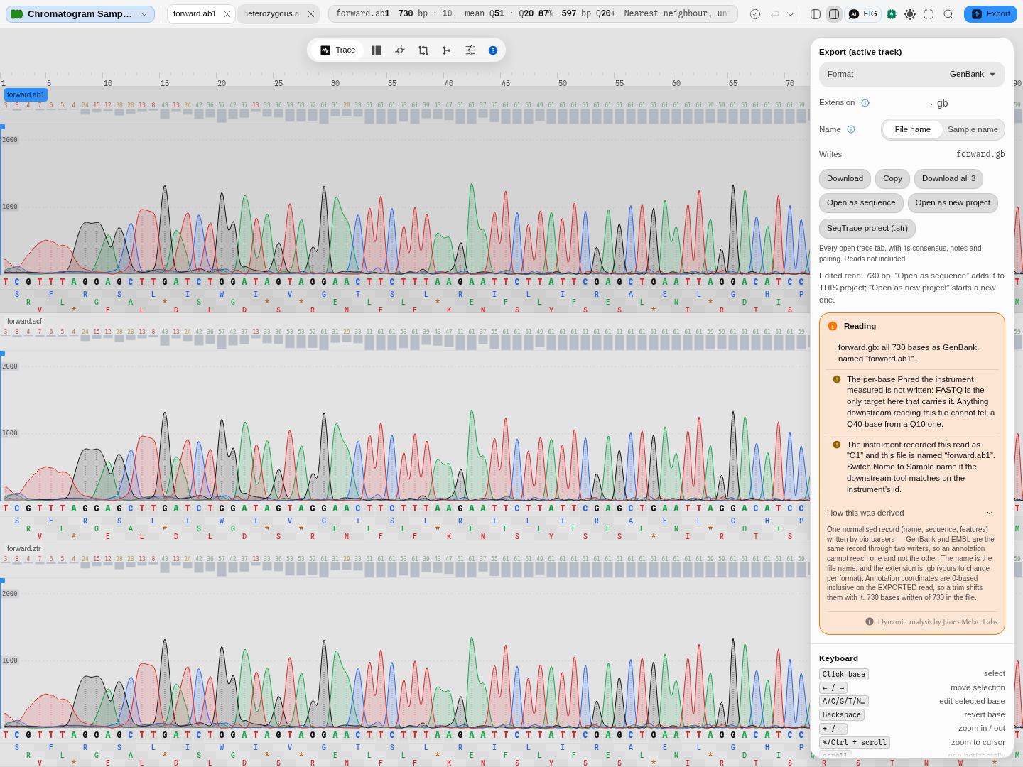
What an export is about to drop, before it is made. All 730 bases of forward.ab1 going out as
GenBank, with two things said that the file itself never would: the instrument's per-base Phred is
not carried by this format (only FASTQ carries it), and the sequencer recorded this read as O1
while the file is named forward.ab1 — so a tool that matches on the instrument's id will not find
it under this name. The fold underneath names the writer, the coordinate convention annotations are
written in, and how many bases of the file reached the record.
Related
Feeds it: a sequencing facility's .ab1, .scf or .ztr; the file manager.
Follows it: Compare Traces to Reference, which takes the trimmed, corrected read and tells you how it differs from a reference; Sequencing Verification, which grades reads against an intended construct; Multiple Sequence Alignment, which takes the tab's tracks as an alignment.
Compare with: nothing else here reads a trace. This is the only surface that shows the four channels.
In this group: Map reads to a reference · Fragment analysis · Alignment · Variant Calls · Population genetics: allele frequencies, Hardy–Weinberg, Fst, linkage disequilibrium · RNA-seq: differential expression with DESeq2, over-represented gene sets, gene set enrichment · Multiple Sequence Alignment · Compare Traces to Reference · Sequencing Verification · Screen for vector contamination
Images
Open a gel photo, micrograph, plate scan or figure beside the data it belongs to, including 16-bit scientific TIFFs a browser cannot decode.
Map reads
Put sequencing reads (DNA or RNA, short or long, single or paired) or assembled contigs where they came from on a reference, and get the alignment back as SAM, with every read's position, strand, mapping quality and alignment.