
Multiple Sequence Alignment
Align a set of sequences and read the result as an alignment you can navigate: per-sequence identity, column conservation, and the scores that quantify the alignment.
| Reached by | Tools → Multiple Sequence Alignment |
| Formats | FASTA in and out CLUSTAL (.aln) in and out GenBank in |
| Sample project | Alignment sample |
What it does
Takes a set of sequences that are not aligned and works out, column by column, which residues correspond to which — inserting gaps where one sequence has material the others do not. What you get back is a grid: every input as a row of the same width, a consensus, a conservation track, and per-row identity against that consensus.
Two aligners are offered, and they answer different questions. Neither is a fallback for the other, so the choice is yours to make rather than a setting to leave alone — see Algorithms you can choose.
When you’d use this
Used in: Align a set of homologues and build a tree from it
What this computes
Two aligners, not two settings of one. Progressive builds a guide tree from Feng-Doolittle distances over every optimal pairwise alignment and merges most-similar-first under once a gap, always a gap. Partial-order aligns into a graph rather than a grid, keeping every path the inputs took through it, and derives its consensus from the graph rather than by column majority.
Per alignment
- Column count, overall identity and gap fraction
- A consensus, exportable as FASTA, to the clipboard, or as a new project with gaps and uncovered positions removed
- A conservation track per column
- The guide tree (progressive) as a drawing and as Newick, so you can read which merges the alignment's early — and most trusted — decisions rest on
- The alphabet, detected and stated — protein, DNA or RNA — with the counts measured accordingly: residues and amino-acid identity for protein, bases for nucleotide
- Alignment-quality scores, graded with a matrix separate from the one that shaped the alignment
Per row
- Identity against the consensus, measured only over columns where both carry a residue
- Coverage — how much of the alignment the row spans
- Substitution and gap counts that never overlap, so they add up
- A pairwise check: the row's identity to its closest row in the alignment, beside the identity of the same pair aligned on its own (optimal, end gaps free, checked against biotite). A row the alignment holds out of register, past the box-plot outlier fence of this run's differences and outside the pair's own 95% interval, is flagged by name with the setting that keeps it together. On 19 HIV-1 env genes under global partial-order alignment, the 768 bp vi557 fragment reads 67.1% to its closest row against 81.6% as a pair
Guide-tree clustering is four published rules, not a cosmetic choice: UPGMA (a molecular clock), neighbour-joining (no clock, corrects for rate differences), BIONJ (NJ with variance weighting) and WPGMA (each merged group counts equally). Same sequences and same distances, a different merge order — on eight cricket COI genes, neighbour-joining gives a 606-column alignment where UPGMA gives 609.
The consensus secondary structure a file states, read and measured. A Stockholm alignment can
carry a #=GC SS_cons line — the consensus RNA fold the family is built around, written in WUSS, the
bracket-and-letter notation Rfam and Infernal use. Two readouts sit above the residues, and they
answer different questions:
- The structure line is what the file asserts: which columns pair with which, and what each unpaired column is — hairpin loop, bulge or interior loop, multifurcation, external single-stranded region, insertion, or a local end where the data simply stops. Pseudoknots are read as pseudoknots: in WUSS they are written as letter pairs precisely because they cross a bracketed stem, and a reader that treated them as brackets would silently drop them.
- Pair support is what the rows do about it: per pair, the fraction of sequences whose two bases actually form a Watson–Crick or GU wobble pair — the pair set covariance models score. It turns a published structure from an assertion into a measurement. On the Rfam tRNA seed, 954 sequences support the 21-pair cloverleaf in a median 98% of rows; a family whose annotation is not borne out reads low here, and the histogram says which stems are the weak ones.
The pair table is read against ViennaRNA, glyph by glyph, including the strings it refuses.
SS_cons is two alphabets, and the wrong one is refused by name. Pfam writes protein secondary
structure into the same field, in DSSP states — H/G/I for helix, E/B for strand, T/S/C for everything
else. Those letters are legal WUSS pseudoknot openers, so parsing a Pfam alignment as RNA would draw
base pairs for a protein. The structure lanes do not appear, and the alignment says which alphabet it
found and why there is nothing to pair.
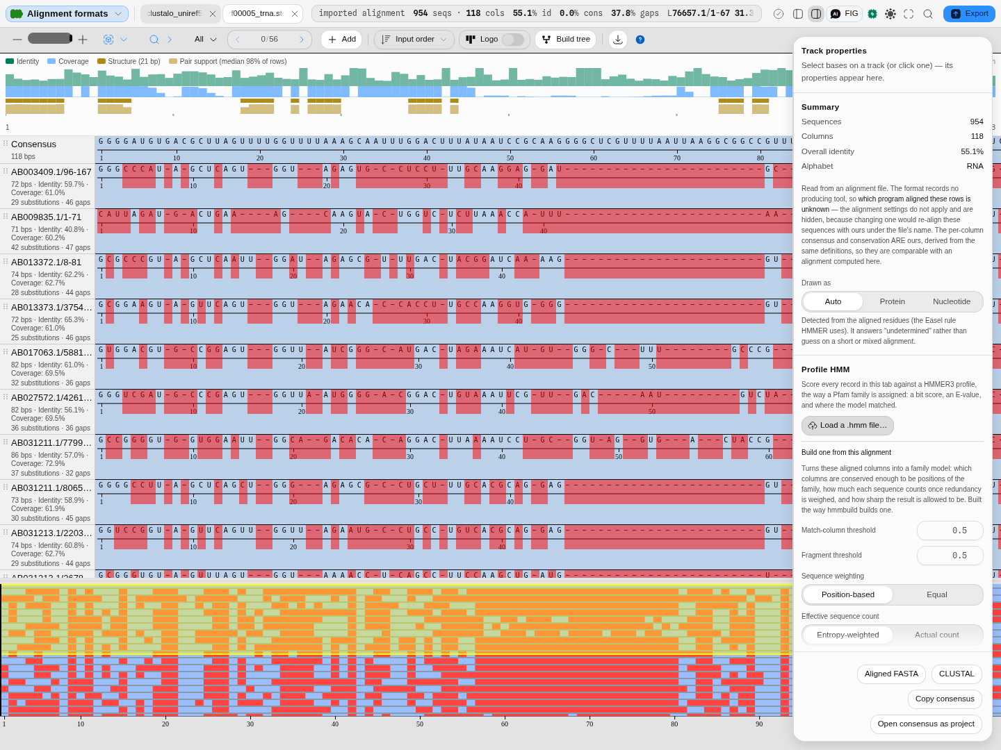
Profile HMM screening answers a different question — does this sequence belong to this family — against a HMMER3 model rather than another sequence, so it weights each position by what that family actually tolerates. You can screen against a published Pfam model or build one from the alignment in front of you.
Imported alignments are shown, never re-aligned. The alignment settings are hidden for a file somebody else produced, and where the format records the producing program — a CLUSTAL header always does, a GCG MSF header sometimes — the viewer names it, and where the format records nothing (aligned FASTA, PHYLIP, Stockholm) it says the producer is not recorded rather than naming the file format as though it were the aligner.
Every number says what it was measured over. Above the readouts the panel states the alignment in one line — how many sequences, how many columns, the mean identity and how many columns are identical in every row — and then the chain behind it, each link openable:
- the identity, and its denominator: the share of the covering rows that carry the column's majority residue, averaged over columns and weighted by how many rows reach each one, with columns no row covers excluded and gaps never counted as agreement;
- the consensus rule, over the input rows only, and how many columns are all gaps;
- the aligner and its own parameters — for the progressive engine the matrix it actually used
(naming which one
Autoresolved to), the gap model with the numbers in force, and the merge order in Newick; for partial-order, the mode and the three scores; - the alphabet, and where the answer came from — declared by the source records, detected by Easel's rule, or forced by you;
- the quality scores, or the reason there are none;
- the inputs, with their ungapped lengths, so a row that spans part of the alignment is visible as a length rather than inferred from a low identity.
Cautions are measured, not judged. A row spanning less than half the alignment is named with the share it covers; a substitution matrix that cannot score these residues is named with the engine's own reason; a protein matrix over a nucleotide alignment is named as what it is — BLOSUM62 reads A, C, G and T as alanine, cysteine, glycine and threonine and returns a number with no error raised. None of these is a threshold anybody invented: each states a measurement and leaves the judgement to you.
What it refuses, with the reason: fewer than two sequences with content; a residue the chosen substitution matrix does not score, named with its position; a pair too divergent for a distance to exist; a gap penalty entered as a positive number, caught beside the box you typed it in; and a consensus-structure line written in protein DSSP states rather than RNA notation, which is named as what it is rather than drawn as base pairs.
Where it lives
Open it from Tools → Multiple Sequence Alignment, from the command palette, or by opening an alignment file already in the project — a CLUSTAL, Stockholm, PHYLIP, GCG MSF, A2M or aligned-FASTA file opens straight into this canvas rather than as text.
It is a canvas, not a rail panel: the alignment gets its own tab beside the map and the sequence view, and it stays there. Each tab holds its own sequences, its own aligner and its own options, so two alignments can be open side by side and compared without either losing its settings — and both survive a reload, because the tab records the question (which rows, which options) rather than the result.
The inspector on the right belongs to whatever you select: click a row and it describes that sequence against the alignment; click nothing and it describes the alignment as a whole.
It hands off, both ways. Build tree sends the aligned rows — never the generated consensus — to Phylogenetics, and the consensus can be opened as its own project to carry into primer design, annotation or a further alignment.
Inputs and outputs
In. Two or more sequences — records from the files in your project (FASTA, GenBank, Swiss-Prot and the rest), a selection, or pasted bases. Nucleotide or protein; the alignment works out which and says so.
Adding sequences from your project. Add → Project files lists every sequence record in the project, grouped under the file it came from, with its length beside it. A multi-record file — a multi-FASTA, a multi-record GenBank — is expanded, so you tick the individual records you want rather than the whole file: eight cricket COI genes in one file are eight rows, not one. Records already in this alignment are marked added and cannot be picked twice, so you can come back to the list and top it up without hunting for what is already there.
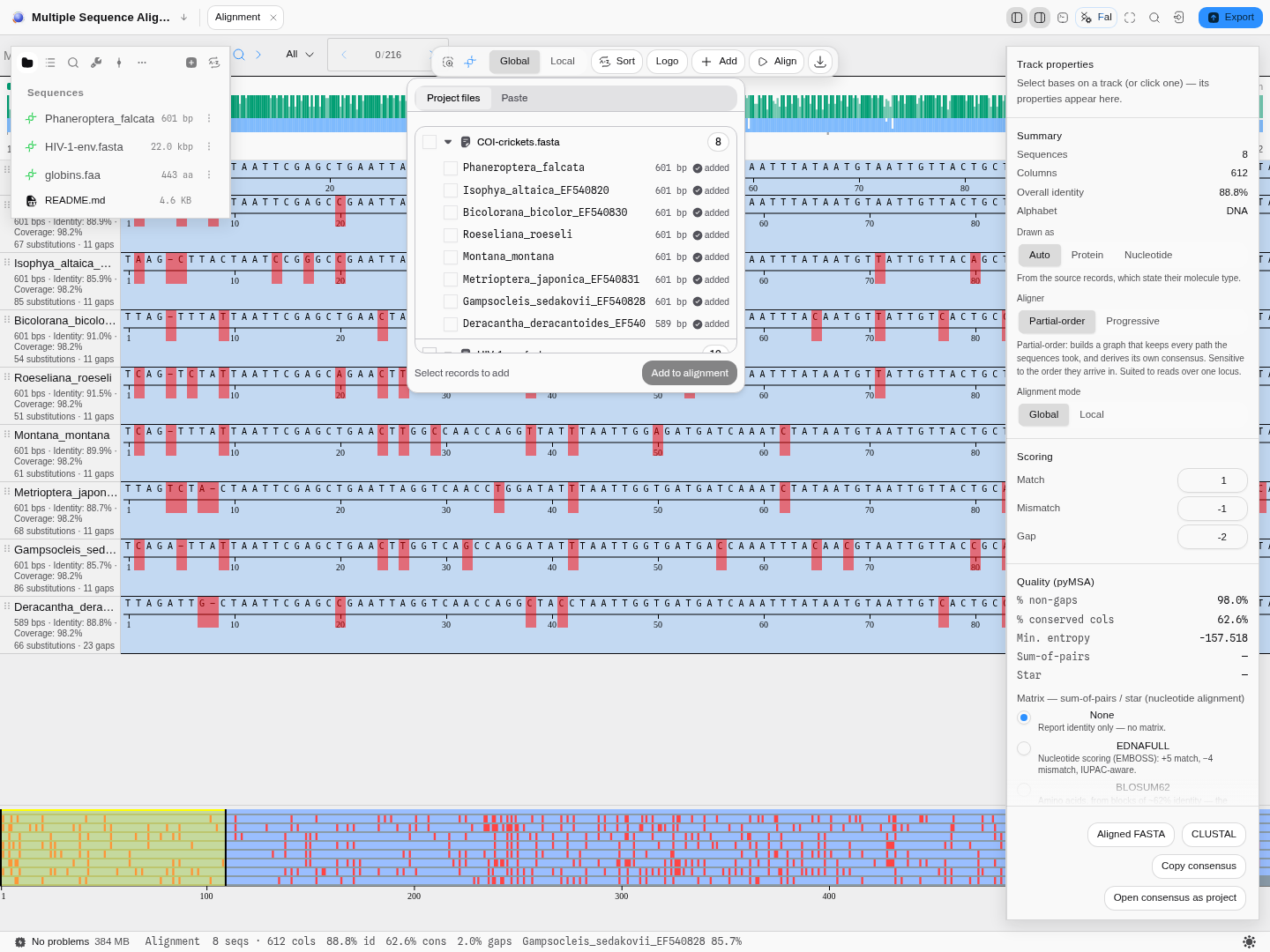
The list is built from each file's record index and lengths, and only the records you tick are read in full. In practice that means the list appears immediately on a project of any size, and picking two records out of sixty costs two reads rather than sixty — worth knowing when you are working from a project of whole-genome or multi-megabase files, where the difference is the one between an instant list and a stalled tab.
Also in: alignments somebody else made. CLUSTAL, Stockholm, PHYLIP, GCG MSF, aligned FASTA, A2M
and A3M files open directly in the viewer. They are shown, never re-aligned — the alignment
settings are hidden for an imported file, because changing one would silently replace another
program's result with ours under its own name. Where the file records which program produced it, the
viewer names that program: a CLUSTAL header always does, and a GCG MSF header does when a program
such as PileUp wrote the file. An MSF written by EMBOSS starts with the format's own
!!AA_MULTIPLE_ALIGNMENT line, which names no aligner, so nothing is claimed for it. Where the
format records nothing at all — aligned FASTA, PHYLIP and Stockholm carry no such field — the viewer
says the producer is not recorded rather than naming the file format as though it were the aligner.
Out. Aligned FASTA, CLUSTAL, the consensus as FASTA or to the clipboard, the guide tree as Newick, and the consensus as a new project — one click to carry it forward into primer design, annotation, or another alignment. Gaps and uncovered positions are removed, so what you get is a real sequence; the project note records how many sequences it came from and which aligner made it.
What it refuses, and what it says. Fewer than two sequences with content in them; a residue the chosen substitution matrix does not score (named, with its position); and a pair of sequences too divergent for a distance to exist. A gap penalty entered as a positive number is caught before the run, beside the box you typed it in.
Demo
Silent, 20 seconds, recorded on the bundled Alignment sample. Eight cricket COI genes arrive aligned by the partial-order aligner: 612 columns, 88.8% mean identity, 383 columns identical in every row. How this was derived opens the chain behind that sentence (the identity measure, the consensus rule, the aligner and its inputs). Switching the aligner to Progressive realigns the same sequences, and Build tree hands the alignment to Phylogenetics. The worked example above gives the numbers each step produces.
Worked example
Open the Alignment sample project. It seeds a Multiple Sequence Alignment tab on eight bush- cricket COI genes (589–601 bp, 85–95 % identity between them).
| Do this | You get |
|---|---|
| As it opens — Partial-order, Global | 612 columns, 88.8 % overall identity, 2.0 % gaps |
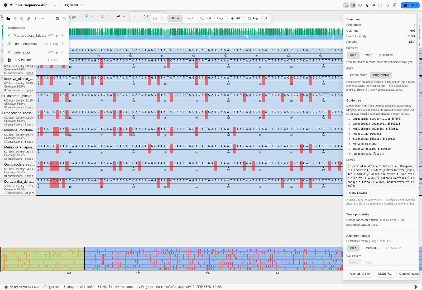
| Aligner → Progressive (matrix Auto → EDNAFULL, linear −10) | 609 columns, 88.9 % identity, 1.6 % gaps, and a guide tree that merges Deracantha and Gampsocleis first |
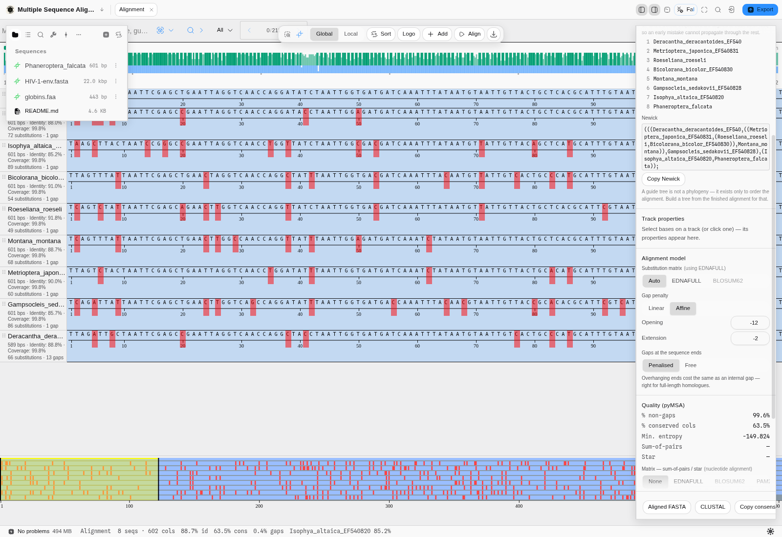
| Gap penalty → Affine (−12 open, −2 extend) | 602 columns, 0.4 % gaps — each row drops from eight gaps to one, because the affine penalty keeps an indel together instead of scattering it |
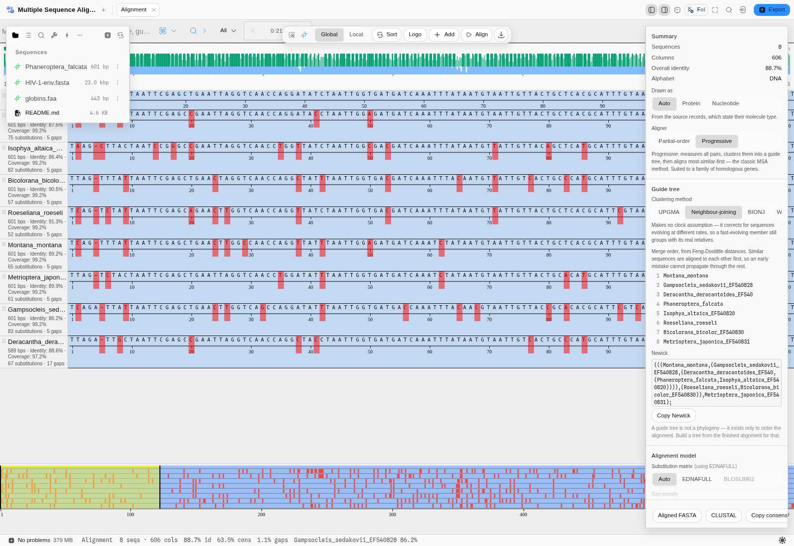
| Guide tree → Neighbour-joining (back on the linear penalty) | 606 columns, and a different merge order — same sequences, same distances, different clustering |
Read the per-row captions as you go: 601 bps · Identity: 89.7 % · Coverage: 98.7 % · 62 substitutions · 8 gaps. Identity is measured over the columns where that row and the consensus both
carry a residue; coverage is how much of the alignment the row spans; substitutions and gaps never
overlap, so they add up.
Controls
Aligner
Chooses between the two methods described in Algorithms you can choose. Changing it re-runs the alignment and replaces the options below it with that method's own, because the two do not share parameters.
Substitution matrix (progressive)
Which model of residue similarity the alignment itself is scored with. Auto reads the alignment's alphabet and picks EDNAFULL for nucleotides or BLOSUM62 for amino acids, and states which one it chose. The matrix that does not match your alphabet is offered but disabled, with the reason: BLOSUM62 on DNA would score A, C, G and T as alanine, cysteine, glycine and threonine and return a number that means nothing.
This is a different setting from the matrix used for the quality scores further down the panel — one shapes the alignment, the other only grades it afterwards.
Gap penalty (progressive)
Linear charges the same amount for every gap column. Affine charges more to open a gap than to extend one, which is the biologically motivated choice: a single insertion or deletion of twelve bases is one evolutionary event, not twelve, and a linear penalty scatters it into several short gaps instead of one long one.
The effect is easy to see and worth seeing once. On the eight cricket COI genes, switching from linear (−10) to affine (−12 open, −2 extend) takes the alignment from 609 columns to 602, and each row from eight gaps to one.
Guide tree — clustering method (progressive)
Which rule clusters the pairwise distances into the order the alignment is built in. The distances themselves are the same either way, so this changes only the order — which is what makes it worth trying both.
| Method | Assumes | Reach for it when |
|---|---|---|
| UPGMA (default) | A molecular clock: every sequence evolving at the same rate | Your sequences are a close, evenly-evolving family |
| Neighbour-joining | No clock; it corrects for rate differences | One member evolves much faster than the rest — under UPGMA it gets pushed to the outside for the wrong reason |
| BIONJ | As NJ, with variance weighting | Distances are large or unevenly estimated, i.e. a divergent set |
| WPGMA | Each merged group counts equally, whatever its size | You do not want a large cluster to dominate the averaging |
It is not a cosmetic choice. On the eight cricket COI genes, neighbour-joining produces a 606-column alignment where UPGMA produces 609, from the same sequences and the same distances.
Gaps at the sequence ends (progressive)
Penalised charges an overhanging end like any other gap — correct when your sequences are full-length homologues that ought to line up end to end. Free charges nothing for them — correct when a sequence covers only part of the region, such as a read against a gene, where being short is not a difference.
Guide tree (progressive)
Not a setting but a readout: the order the aligner merged your sequences in, and the same tree in Newick form, which you can copy into a tree viewer. Reading it tells you what the aligner thought was most similar to what — and therefore which parts of the alignment rest on the most confident decisions.
Alignment mode (partial-order)
Global aligns the sequences end to end; Local aligns the best-matching region and lets the rest hang. Match, mismatch and gap scores are set directly here rather than through a matrix.
Alphabet — protein, DNA or RNA
The viewer reports which alphabet your alignment is in, and measures it accordingly. A protein
alignment counts residues (AAs), reports amino-acid identity and the number of identical
positions for each row against the consensus, and offers the amino-acid property colourings; a
nucleotide alignment counts bases and offers the DNA ones.
Where the answer comes from, in order:
- Your files, when their format states it. GenBank, Swiss-Prot and
.xdnarecords declare whether they hold a protein, and that declaration is used as-is. - The residues themselves, for the alignment formats that record no alphabet at all — CLUSTAL, Stockholm, PHYLIP, GCG MSF and aligned FASTA all just hold letters. The rule applied is the one HMMER uses, and it is deliberately conservative: it classifies every row, and when the rows agree that verdict stands. When they disagree it falls back to the composition of the alignment as a whole rather than refusing outright — so a set that mixes a protein and a nucleotide row still gets an answer, drawn from the letters actually present. Undetermined is reserved for the case where even that is not enough evidence: a very short alignment, or one made only of gaps and ambiguity codes. An undetermined alignment is drawn as nucleotide.
- Your override. Drawn as → Auto / Protein / Nucleotide forces it either way, per alignment. The line under the control always states which of the three routes produced the current answer.
Degenerate bases (R, Y, N, W, …) do not make a nucleotide alignment look like a protein: a
consensus full of ambiguity codes is still read as DNA.
Algorithms you can choose
Aligner → Progressive or Partial-order. They are not two settings of one method; they are two methods, and they are good at different things.
Progressive (guide tree)
The classic multiple-alignment method, and the one to reach for when your sequences are a family — orthologues of a gene, members of a domain, variants of a genome.
It runs in three stages:
- Every pair is aligned optimally, and the score of each pairwise alignment is converted into a distance using the method of Feng & Doolittle. That conversion is what makes the numbers comparable: a raw score depends on how long and how similar the two sequences are, so it is normalised against the best either sequence could score against itself and against the score two sequences of the same composition would get by chance.
- Those distances are clustered into a guide tree, which is simply an ordering: which sequences are most alike, and therefore which should be aligned to each other first. Four clustering rules are offered — see Guide tree.
- The alignment is built up along that tree, most-similar-first, following the rule once a gap, always a gap — once two sequences have been aligned, the gaps between them are fixed, and later sequences are fitted around them.
The order matters because an alignment mistake made early propagates. Starting with the two most similar sequences — where you are least likely to be wrong — is the whole idea.
Partial-order
Aligns into a graph rather than a grid, keeping every path the input sequences took through it. Reach for it when your inputs are reads over one locus rather than a family: it is built for the case where sequences genuinely diverge into alternatives, and it produces its own consensus from the graph rather than by taking a column majority.
It has no guide tree and it is sensitive to the order the sequences arrive in, which is the price of representing alternatives faithfully.
Which to pick
| Your input | Reach for |
|---|---|
| Orthologous genes, a protein family, related genomes | Progressive |
| Sequencing reads over one region, or anything where you care about alternative paths | Partial-order |
| You want the result a reader coming from Clustal or MUSCLE would expect | Progressive |
Screening against a profile HMM
The two aligners above answer how do these sequences relate to each other. A profile hidden Markov model answers a different question: does this sequence belong to this family — where the family is not another sequence but a statistical model built from hundreds or thousands of known members.
That difference matters because a pairwise or multiple alignment treats every position alike. A profile does not. It has learned, position by position, which residues that family tolerates and which it never accepts, and how often it inserts or deletes there. A glycine that is invariant across 5,000 kinases counts for far more than one in a loop that varies freely — and only a profile knows which is which. This is why profile methods find remote homologues that a pairwise search misses entirely.
What you need
A profile in HMMER3 format (.hmm). Pfam publishes one for every family it curates. Drop it
into your project like any other file and it appears in the panel's Profile HMM section; models
you keep elsewhere can be loaded from disk instead. If the family you care about has no published
model, you can build one from the alignment in front of you — see Building a profile from your
own alignment below.
The Alignment sample project ships Pfam's own PF00069 (Protein kinase domain) together with four real human proteins, so the whole workflow is one click from the lobby.
Reading a screen, step by step
-
Open the records you want screened as an alignment. In the sample project: FILES →
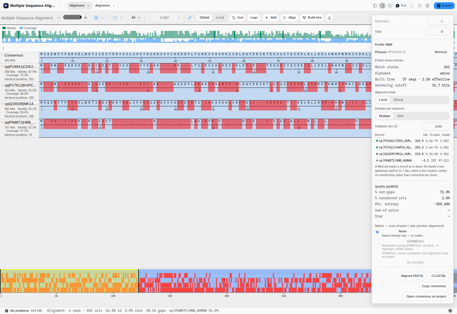
kinase-queries.fasta→ Multiple sequence alignment… → Align. Four proteins, 402 columns. -
Load the model. Rail → Profile HMM →
PF00069_Pkinase.hmm. The readout confirms what was read: 262 match states, alphabet amino, built from 37 sequences (2.56 effective), and a gathering cutoff of 31.7 bits. -
Read the table. One row per record, best first:
Record bits E-value model CDK2_HUMAN 260.9 6.3e-79 1–262 KAPCA_HUMAN 253.3 1.4e-76 1–262 MK14_HUMAN 215.0 6.3e-65 1–262 HBB_HUMAN −3.2 232 97–113 The three kinases each match the model over its full length, 1–262. Haemoglobin matches 17 states out of 262 and scores below zero — the model fits it worse than the background does.
-
Trust the cutoff, not your eye. A filled dot marks a record at or above the family's own gathering cutoff, the threshold the family's curators set as the boundary of membership. Using it beats picking an E-value threshold yourself, because it was chosen by people looking at that family's real false positives.
The controls, and what each one changes
Alignment mode — Local or Glocal. Local looks for the model anywhere inside the sequence and is what a database search does: right when the family is a domain inside a longer protein, which is the usual case. Glocal requires the whole model to align, though the sequence may run past it: right when you are asking whether a record is a full-length family member rather than whether it merely contains the domain. A truncated or fragmentary record scores well locally and badly glocally, and that contrast is the useful signal.
Domains per sequence — Multiple or One. Many proteins carry the same domain more than once. Multiple lets the model match several times and sums the evidence; One scores the single best occurrence. If you are asking "how many copies", use Multiple; if you are ranking candidates for membership, One is the cleaner comparison.
Database size (Z). An E-value is a bit score converted into "how many hits this good would I expect by chance in a database of this size", so it depends on the size you name. Searching 1,000 sequences and searching a million gives the same bit score and E-values a thousand-fold apart. The bit score does not depend on Z — when you want a number that means the same thing tomorrow, quote the bits.
Pitfalls worth knowing
- A nucleotide record against a protein model is refused, and it has to be. Every DNA base is also an amino-acid letter — A alanine, C cysteine, G glycine, T threonine — so a gene screened against a protein family produces a complete table of scores that mean nothing at all, with no error anywhere. The panel checks the molecule type before it runs and says so.
- A model you build here gets its own E-values. The score statistics are fitted by simulation at build time, the same way HMMER does it, so a profile you made yourself reports E-values and not only bit scores. If you switch the fit off, bit scores are still exact and the E-value column says it has nothing to show rather than printing a number it cannot compute.
- Bits below zero are not "a weak hit". They mean the background model explains the sequence better than the family does. Haemoglobin's −3.2 is not a faint kinase.
- A high score over a short span is a domain, not a family assignment. Always read the model span next to the score: 1–262 and 97–113 are very different claims.
Building a profile from your own alignment
Pfam has a model for its families. It does not have one for your family — the twelve homologues you pulled out of a new genome, the variant set from one experiment, the sub-clade nobody has curated. Building a model from the alignment you already have turns that set into something you can screen new sequences against, and it takes one click.
What building actually does, because the three controls are the whole method:
- It decides which columns are positions of the family. A column where most sequences have a residue is a real position; a column that is mostly gaps is an insertion some members happen to carry. Only the former become states of the model.
- It decides how much each sequence counts. Twenty near-identical members carry roughly one sequence's worth of information between them, so they are down-weighted; a divergent member that nobody else resembles carries far more, and is weighted up. Without this, whichever sub-family you happened to sample most heavily becomes the model.
- It decides how sharp the model is allowed to be. Counts are scaled down until the model carries a target amount of information per position. This is the step that separates a family model from a memory of your alignment: a model fitted tightly to the sequences you have will recognise those sequences and little else.
Step by step, on the sample project
- Open an alignment. The Alignment sample project opens on eight cricket COI genes — 612 columns, 88.8% identity. Any alignment in the tab works.
- Open the rail's Profile HMM section and read the block titled Build one from this alignment.
- Set the match-column threshold. The default of 0.5 keeps a column when half the sequences have a residue there. Raise it towards 0.7 to keep only the well-populated columns; lower it to keep gappy ones. On the crickets, 0.7 keeps 597 of 612 columns.
- Choose the sequence weighting. Position-based is the one to use unless your set is already balanced by hand — it is what stops redundancy from voting twice.
- Choose the effective sequence count. Entropy-weighted is the default and the right answer almost always. Actual count builds the sharp, over-fitted model described above, which is occasionally what you want when the alignment IS the population.
- Optionally set the target bits per position. Left blank this is 0.59 for protein and 0.62 for nucleotide. Raising it makes a more specific model that misses more remote members; lowering it makes a more permissive one.
- Leave E-value statistics on Fit. This is the step that lets the finished model report E-values. It scores a few hundred random sequences against the model and fits the score distributions, which takes a fraction of a second and is what HMMER itself does at the end of every build. Skip is there for when you only ever intend to compare bit scores.
- Press Build profile. The model loads immediately and every record in the tab is scored against it. On the crickets at threshold 0.7 and a 0.8-bit target: 597 match states, an effective count of 3.07 of 8 — the eight crickets carry about three sequences' worth of independent information — and 0.80 bits per position, the target it was asked for. The report also names the fitted statistics: lambda 0.69616, MSV mu -11.8152, Viterbi mu -12.1556 and Forward tau -6.7769. Every record then scores between 737 and 776 bits against its own family, with E-values from 1.2e-222 down to 2.1e-234.
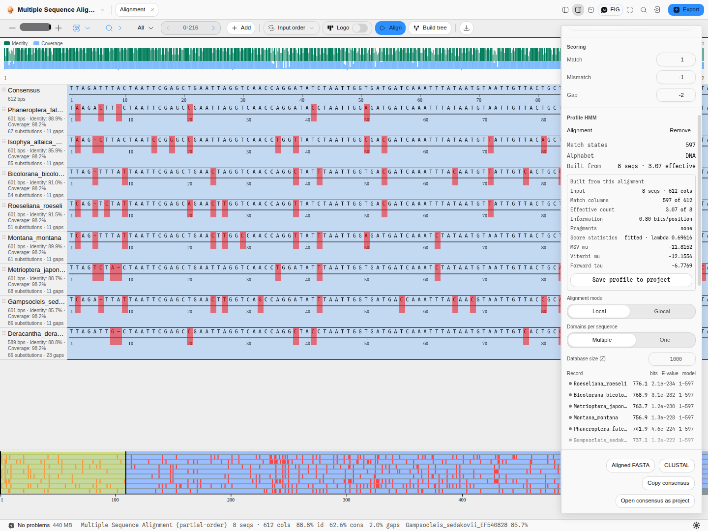
The report under the model is worth reading rather than skipping: match columns tells you how much of your alignment became model, effective count tells you how redundant your set really is, information tells you how sharp the result is, and fragments names any sequence short enough that its missing ends were treated as unknown rather than as deletions — which is what stops a partial sequence from teaching the model gaps that were never there.
The score statistics, and why there is only one lambda
A bit score says how much better the family explains a sequence than the background does. Turning that into an E-value — how many sequences this good would I expect by chance — needs to know the shape of the score distribution for sequences that are not members, and that shape depends on the model. Fitting it is what the Fit setting does.
The report names four numbers, and they are not four independent fits:
- Lambda is the slope of the tail, and it is calculated, not simulated. It follows from the model's own length and information content, with a small correction for edge effects. That is why one lambda is quoted for all three scoring methods rather than three.
- MSV mu locates the distribution for the fast ungapped-match score, the first filter a search applies.
- Viterbi mu locates it for the single best alignment path.
- Forward tau anchors the tail for the score summed over all alignment paths, which is the one the E-value column actually uses.
Two of the three are the outcome of scoring a few hundred random sequences, so they are estimates with a spread of roughly a tenth of a bit — about 8% on an E-value. That is why the bit score, which involves no simulation at all, is the number to quote when you want something reproducible.
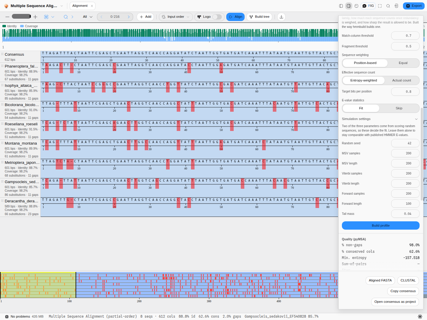
Simulation settings exposes every knob behind that fit. The defaults are HMMER's own, and they are the values every published HMMER E-value was fitted with, so changing one makes your model's E-values incomparable with those. Worth knowing anyway:
- Random seed makes the fit reproducible. The same seed gives the same parameters every time; changing it is the honest way to see how much the estimate moves.
- Samples and length per method trade time for precision. More samples narrows the estimate; the lengths are chosen so the model sees sequences of a realistic size.
- Tail mass is where the Forward tail is anchored from. HMMER's 0.04 is tuned so that two opposite errors cancel, which is a stronger reason to leave it alone than "it is the default".
Pro tips
- Build, then screen the same sequences you built from. They should all score highly. If one does not, it is probably misaligned, and the model just told you so.
- An effective count far below your sequence count means your set is redundant. Three of eight is normal for one genus; three of eighty means you should sample more widely before trusting the model as a family definition.
- A model built from two sequences is not a family model. Two is the minimum accepted, and it is accepted because it is occasionally useful, not because it is good practice.
- Save the model to your project once you are happy with it. It reappears in the same section next session and can be loaded onto any other alignment.
What it hands to the rest of the workbench
Selecting a hit scrolls the alignment to the columns its domain occupies, so the region the model matched is the region you are looking at. The record's coordinates are mapped through its own gaps, so the mark lands on the residues the model actually scored rather than on the raw sequence offsets.
It also reaches the record's own view. Open the record the hit belongs to and the matched domain is drawn on its sequence and linear map, coloured by whether the record cleared the family cutoff, with the score and the span of the model it used in the tooltip. If the record is not open yet, open it whenever you like — the mark appears when it does.
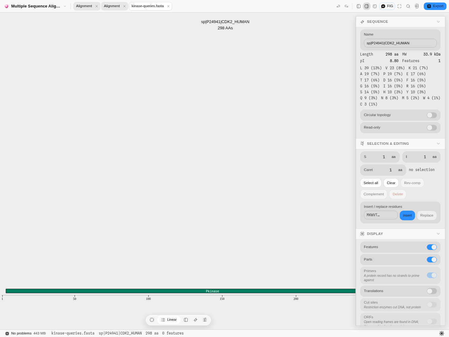
A profile you built is saved into your project like any other file, so it can be screened against a different alignment, exported, and shared with the people who need to reproduce your assignment.
The science
The distance between two sequences (progressive aligner) is
$$D_{a,b} = -\ln!\left(\frac{S_{a,b} - S^{rand}{a,b}}{S^{max}{a,b} - S^{rand}_{a,b}}\right)$$
where $S_{a,b}$ is the optimal pairwise alignment score, $S^{max}$ is the mean of the two self-alignment scores — the best the pair could possibly do — and $S^{rand}$ is the score expected from sequences of the same length and composition aligned at random, plus the gap penalties the real alignment actually paid. Two sequences that align no better than chance have no defined distance, and the tool says so rather than reporting a number (see Limitations).
Feng, D. F. & Doolittle, R. F. Progressive alignment of amino acid sequences and construction of phylogenetic trees from them. Methods in Enzymology 266, 368–382 (1996).
The pairwise alignments underneath are exact — full dynamic programming (Needleman–Wunsch with a linear gap penalty, Gotoh with an affine one), not a heuristic. Every optimal alignment is found; where several score identically, one is chosen by a fixed, documented rule so that the same input always gives the same answer.
The substitution matrices are the standard published ones: EDNAFULL (EMBOSS NUC.4.4, Todd Lowe
1992) for nucleotides, including the IUPAC ambiguity codes, and BLOSUM62 for amino acids.
How the results are checked. The progressive aligner is verified against biotite, byte for byte, on the real sequence files this application ships: every one of 929 pairwise alignments across 208 cases — including all 30 cases where more than one alignment scores equally well — every cell of 12 distance matrices to the last bit of precision, and 24 complete multiple alignments. The partial-order aligner is verified the same way against poapy, the alignment-quality scores against pyMSA, and the alphabet detection against HMMER's own Easel library.
Shared with other tools: Alignment scoring compares how every tool that does this chooses its method.
Limitations
- Both aligners are exact, and exact is quadratic. Every pair of sequences is aligned in full, so the work grows with the square of the number of sequences and with the product of their lengths. A few dozen genes is comfortable; a few hundred long genomes is not what this is for.
- Progressive alignment cannot revisit a decision. Once a gap, always a gap is what makes the method tractable and also what limits it: a gap placed early is never reconsidered in the light of sequences added later. Iterative refinement, which repeatedly pulls sequences out and re-aligns them, is not offered.
- Sequences that align no better than chance have no distance. If a pair scores below what its own composition would score at random, the logarithm in the distance formula is undefined and the alignment is refused with that reason, rather than reported with a fabricated number. If you hit this, your set is too divergent to align as one family — split it, or align the parts you know are related.
- The guide tree is not a phylogeny. It exists to order the alignment and nothing more; its branch lengths are a clustering artefact. Build a tree from the finished alignment if you want an evolutionary hypothesis — that is a different tool, and it offers real substitution models.
- The progressive aligner has no profile-HMM mode. Searching a sequence against a Pfam or Rfam model, rather than aligning sequences to each other, is a separate capability and is not built.
- Every symbol must be in the chosen matrix.
J(leucine-or-isoleucine) is a legal amino-acid code that BLOSUM62 does not score, and the aligner names the symbol and its position rather than quietly reading it as something else.
Compared with other tools
| This alignment canvas | SnapGene | Geneious Prime | |
|---|---|---|---|
| Alignment | Two engines: exact progressive (Needleman–Wunsch / Gotoh, four guide-tree methods) and partial-order | "Pairwise and multiple DNA and protein alignment, alignment to a reference" | "Pairwise and multiple alignment of DNA or protein" |
| Guide tree | Drawn, with the clustering method as a control, and every distance derivable | Not described on the feature page | Not described on the feature page |
| Sanger contigs | Not here — that is the trace tools' job | "De novo contig assembly of Sanger reads using CAP3" | Assembly listed among its tools |
| Profile HMM screening | Built from the alignment itself, in the same canvas | Not listed | Not listed |
Sources, first-party and dated: https://www.snapgene.com/features (retrieved 2026-08-08) and https://www.geneious.com/features (retrieved 2026-08-08), the same feature pages quoted verbatim above.
What they have that this does not: CAP3 de-novo contig assembly of Sanger reads is a real gap on SnapGene's side — the trace tools here align reads to a reference, they do not assemble them into a contig. Both vendors also ship decades of file-format and workflow integration around alignment that no single canvas replaces. And "not described on the feature page" is exactly that: neither vendor publishes an exhaustive list, and neither is runnable here to check.
Export
- Aligned FASTA (
.aln.fasta) — every row with its gaps, wrapped at 60 columns. The interchange format: it reads into any downstream aligner, tree builder or viewer. - CLUSTAL (
.clustal) — interleaved 60-column blocks with the conservation line under each, which is the format to paste into a paper or a lab notebook because it is readable as text. The consensus row is excluded from it, as CLUSTAL expects. - Copy consensus — the consensus sequence to the clipboard.
- Open the consensus as a project, which is how you carry it forward into primer design,
annotation or another alignment. Gaps and the
?characters that mark uncovered positions are stripped, because a project sequence has to be a real sequence; an alignment whose every column is a gap says so rather than opening an empty project. - Build tree hands the aligned rows to Phylogenetics — the input rows only, never the generated consensus, which would put a taxon on your tree that is not a sequence anyone has.
API
@ports/msa — the alignment itself, with no editor state:
import { runMsa } from '@ports/msa';

// Partial-order (the default engine)
const poa = runMsa(rows, { globalAlign: true, matchscore: 4, mismatchscore: -2, gapscore: -4 });

// Progressive: exact pairwise DP under a guide tree
const prog = runMsa(rows, {
  engine: 'progressive',
  alignMatrix: 'EDNAFULL',        // or BLOSUM62 for protein
  gapPenalty: [-12, -2],          // a pair = affine (open, extend); a number = linear
  terminalPenalty: false,         // free end gaps
  guideTree: 'upgma',             // upgma · nj · bionj · wpgma
  scoreMatrix: 'BLOSUM62',        // the matrix the QUALITY scores are graded with
});
rows is { name, sequence }[]. The result carries rows (each with its gapped aligned string
and an isConsensus flag), length, count, consensus, conservation, the per-column facts and
the quality scores. Each engine is handed only its own options, so a POA-shaped knob cannot
silently reach the progressive aligner and read as though it had applied.
RNA is transcribed in and mapped back out: the ported progressive aligner has no U,
faithfully to biotite, so a U sequence is aligned as DNA and restored to RNA on the way out rather
than being refused or silently mis-scored. A row carrying both U and T is deliberately not
transcribed — that is not RNA, and folding the two letters together would score a real difference as
a match — so it keeps the aligner's own refusal by name.
Automation
- Workflow DAG: the node is
align_sequences, categoryread, so it needs no approval. Itssequencesport takes severalsequence/recordinputs at once — protein as readily as DNA — andinclude_subject(default on) adds the node's own subject. - Both aligners, and every option either one takes.
enginechooses partial-order or progressive. The partial-order engine readsglobal_align(on by default, so a full-length comparison is what you get unless you ask for a local one),match,mismatchandgap; the progressive engine readsalign_matrix,guide_tree, the gap model (affine_gapwithgap_open/gap_extend, or a flatgap_penalty) andterminal_penalty.score_matrixgrades the quality report under either. The options and their starting values are the ones the panel opens on, so the same request answered in the panel and in a workflow is the same analysis. - Outputs:
rows(name + gapped sequence),length(columns),count(aligned sequences, excluding the generated consensus),consensus,conservation(the Clustal-style line),engine(which aligner ran),scores(the quality report),guideTreeNewick(the merge order, progressive only), andalignedSequences— the input rows only. Wire that last one intobuild_tree: feedingrowsin put the POA consensus on a four-sequence phylogeny as a fabricated fifth tip, which is the reason the two ports are separate. - Refusal: fewer than two sequences is refused by name, saying how many it got and where to wire more, rather than returning an empty alignment.
- The copilot calls the same tool by the same name with the same parameters.
Provenance
What is versioned is the question, not the answer. The step log records which sequences were aligned, under which options, under what name — the alignment itself is a pure function of those, so storing it would duplicate what can always be recomputed. Restoring a version re-runs it.
Inputs are stored by reference wherever possible: a row that came from a project file keeps that file's id and its length rather than a second copy of the sequence. Only a pasted sequence with nothing behind it is stored verbatim. A referenced file that has since been deleted is reported on restore, never silently dropped or substituted with something else.
An imported alignment says who aligned it, or says that nothing recorded it. CLUSTAL and GCG MSF name their producing program in the file and that name is kept; Stockholm, PHYLIP, A2M and aligned FASTA do not, and the inspector reads "Read from an alignment file. The format records no producing tool, so which program aligned these rows is unknown" rather than naming the file format as though it were a program. A Pfam family id is not lost in the process — it stays in the record's metadata.
Citing the method: name the engine (partial-order, following poapy; or progressive, following biotite), the substitution matrix, the gap penalty and the guide-tree method. Both are checked against those libraries, and the comparison can be re-run.
Screenshots
The progressive aligner on the bundled Alignment sample: 609 columns, the guide tree drawn beside
the rows, and each row captioned with its own identity, coverage, substitutions and gaps.
Affine (−12 open, −2 extend) against linear (−10): 602 columns instead of 609, and one gap per row
instead of eight — the same indel kept together rather than scattered.
Neighbour-joining over the same distances gives 606 columns where UPGMA gives 609. The distances do
not change; only the order the alignment is built in does.
The result of screening a profile built from the aligned rows: the Pkinase hit on human CDK2,
written back onto the record as a feature spanning the columns it matched, so the match is on the
map rather than only in a table.
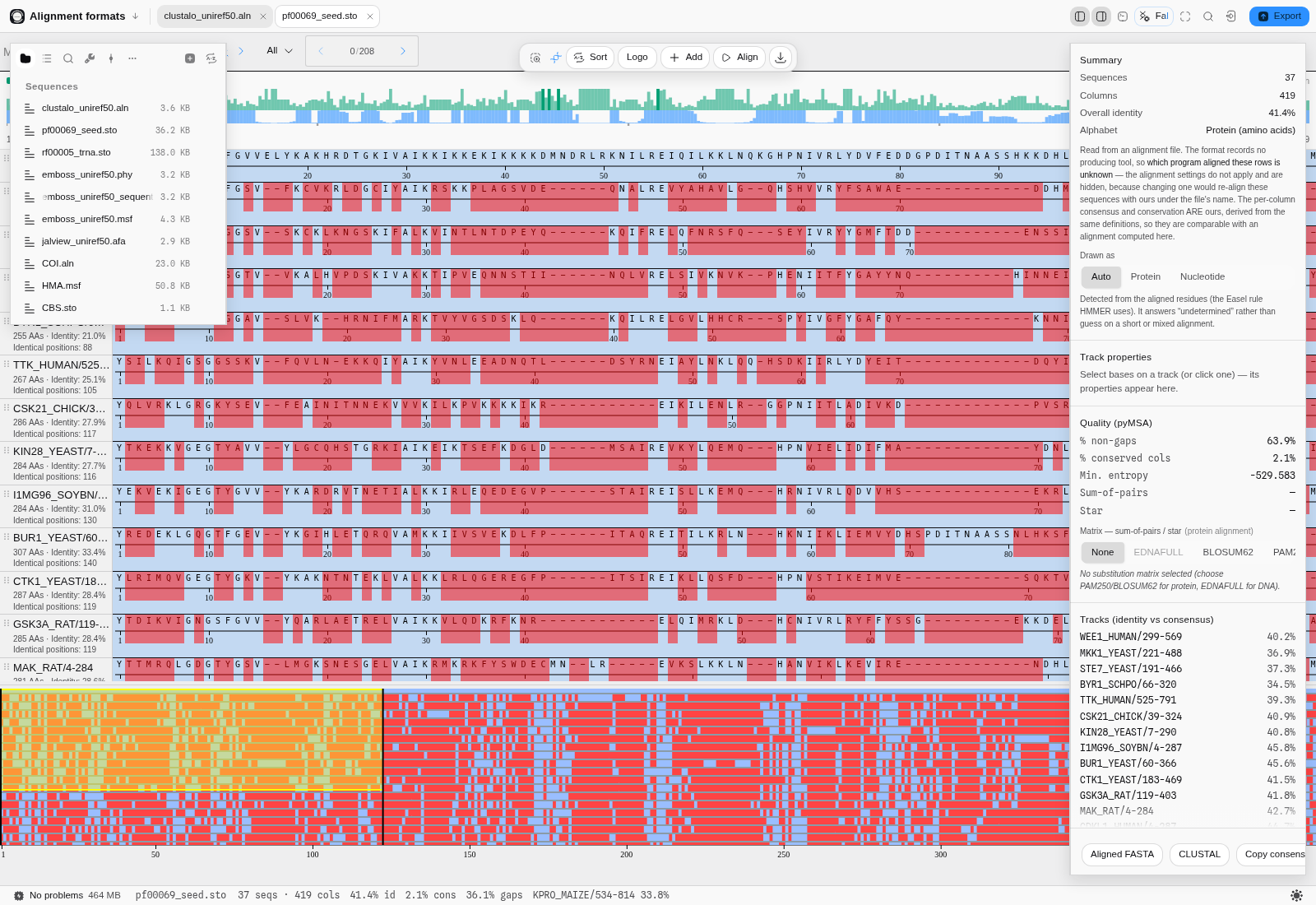
pf00069_seed.sto. Stockholm does not record which program aligned the rows, so the inspector says
so instead of naming the file format as though it were an aligner.
Related
In this group: Chromatogram · Map reads to a reference · Fragment analysis · Alignment · Variant Calls · Population genetics: allele frequencies, Hardy–Weinberg, Fst, linkage disequilibrium · RNA-seq: differential expression with DESeq2, over-represented gene sets, gene set enrichment · Compare Traces to Reference · Sequencing Verification · Screen for vector contamination
RNA-seq
Find the genes whose expression differs between conditions from raw RNA-seq read counts with DESeq2, edgeR's quasi-likelihood test or limma-voom, then ask which gene sets those genes over-represent and which sets sit at the top or bottom of the whole ranking.
Compare Traces to Reference
Grade a plate of Sanger reads against the sequences they were meant to be: a per-column variant table with a conservative consensus, coverage and confidence, codon consequences on either strand, and each read matched to its own reference.