
Phylogenetics
Turn an alignment into a tree, then judge how much of that tree the data actually supports.
| Reached by | Tools → Phylogenetics · Build tree, on any alignment |
| Formats | FASTA in CLUSTAL in Newick in/out NEXUS in/out PhyloXML in/out NeXML in/out SVG out PNG out |
| Sample project | Phylogenetics · Tree files |
What it does
A tree is a hypothesis about how a set of sequences are related, inferred from an alignment. This tool builds one by any of eight methods, puts a number on how much of it the data supports, and gives you the apparatus to interrogate the result rather than just admire it.
The thing worth being clear about up front: a tree is a summary, and summarising loses information. Eight sequences have 28 pairwise distances; the tree that represents them has 13 branch lengths. Those 28 numbers cannot in general be reproduced exactly by 13, so every tree is a compromise, and the interesting question is where the compromise is worst. That is what the Compare tab's input-versus-patristic table is for, and it is the reason the distance matrix stays available after the tree exists.
When you'd use this
Used in: Align a set of homologues and build a tree from it
- "How are these homologues related?" The ordinary case: a gene from several taxa, aligned, then a tree. Neighbor-Joining with bootstrap is the standard first answer and takes about a second.
- "Which of my clones came from which parent?" Sequence variants of one construct are just a small phylogenetic problem. A tree groups them and the support values say which groupings to trust.
- "Does my tree agree with the published one?" Paste or open the other tree in Compare and get Robinson-Foulds, weighted RF, branch score, path difference and the quartet breakdown — plus the explicit list of clades the two trees disagree about.
- "Which substitution model should I even use?" Compare models fits every model with and without rate heterogeneity, ranks them by AIC, AICc or BIC with Akaike weights, and hands the winner to the build.
Reach for something else when: you want to know whether two sequences are related at all rather than how — that is BLAST. If you want to see structural rearrangements rather than a branching order, use the Dot Plot; a tree cannot express an inversion. And if your sequences are not yet aligned, they must be — see Inputs and outputs below, because this is the mistake that silently produces a wrong tree rather than an error.
What this computes
A tree, the support for it, and how much the tree lost — the last being the part most tools omit.
Nine inference methods in four families, each stating whether it assumes a molecular clock: Neighbor-Joining, BIONJ (NJ weighted by each distance's variance), FastME balanced and FastME OLS (minimum evolution with NNI/SPR search), UPGMA and WPGMA (which force an ultrametric tree and therefore do assume a clock), Maximum Parsimony (no substitution model at all, susceptible to long-branch attraction), Maximum Likelihood, and Bayesian (MCMC) (posterior sampling under a strict or relaxed clock with a coalescent tree prior, or with no clock on an unrooted tree).
The clock column is not decoration. UPGMA and WPGMA make every tip equidistant from the root, which is right only if all lineages evolve at the same rate; when they do not, UPGMA does not merely lose accuracy, it can recover the wrong topology. That assumption sits next to each method rather than in a footnote.
Per run
- The tree — topology and branch lengths — and the distance matrix it was built from, kept available afterwards rather than discarded
- Support, by bootstrap, aLRT, aBayes or SH-aLRT — different questions about the same branch, described below — and the bootstrap itself reports either the Felsenstein proportion (FBP) or the transfer bootstrap (TBE), two statistics read off one set of replicates. The bootstrap is re-inferred by the method that produced the tree — a likelihood analysis bootstraps under likelihood, a parsimony analysis under parsimony. This matters more than it sounds: resampling the columns and then re-inferring each replicate with a distance method would give you support values that say how often Neighbor-Joining recovered each clade, which is a different question about a different estimator, reported against your tree. The replicate count you chose is therefore also a cost: N replicates is N full searches under parsimony and N full optimisations under likelihood. The three searches on offer are all hill climbs from the NJ tree and all return a local optimum; SPR can cut a clade out and graft it elsewhere, which lets it leave an optimum NNI cannot — measured on this app's own samples, 974 steps against 975 on 18 cricket COI barcodes and 2,133 against 2,161 on 25 HIV-1 env genes — and TBR can also turn that clade around before regrafting it, widening the sweep from 842 candidate trees to 1,874 on those same 18 barcodes. A bootstrap re-runs the whole search per replicate, so SPR at 100 replicates is 100 searches, and the panel warns rather than looking hung
- Input distance against patristic distance, pair by pair. Eight sequences have 28 pairwise distances and their tree has 13 branch lengths, so 28 numbers cannot in general be reproduced by 13 — every tree is a compromise, and this table is where the compromise is worst
- The alignment diagnosed before any tree is built, because a tree from a bad alignment is a confident wrong answer
Per Bayesian run, in place of a support method:
- Clade posterior probability — the share of the sampled trees that contain each clade, printed on the majority-rule consensus of those trees (clades in at least half of them)
- Node heights on that consensus: each node sits at its clade's mean height over the samples that contain it, the convention BEAST's TreeAnnotator uses, so the summary tree is ultrametric; each clade also reports its height's 95% highest posterior density (HPD) interval
- Every clade the chain visited, including those too rare to draw, and the most probable topologies with their posterior shares
- Trace summaries for the log posterior, the log likelihood, theta (4Nμ) and the root height: posterior mean, 95% HPD interval and effective sample size (ESS), flagged below 200, Tracer's threshold for a chain too correlated to trust
- The maximum a posteriori (MAP) state the chain visited, and each move's acceptance rate
- With no clock: the tree is unrooted, each clade is one side of a split, the clade table gives the mean length of the split's branch with its 95% HPD, and the tree length (the sum of all branch lengths) replaces theta and the root height in the traces and the convergence check
- Under the relaxed clock: the posterior of the clock's sigma (the log-scale standard deviation of branch rates), and of the branch rates' coefficient of variation and mean, each with its 95% HPD interval and ESS; every sampled parameter joins the low-ESS warning
- Convergence across independent runs, when you ask for two or more: the runs start from different seeds, their samples are pooled for everything above, and two diagnostics say whether they found the same posterior. The average standard deviation of split frequencies (ASDSF) takes every clade some run sampled in at least 10% of its trees (the share is yours to set) and averages the standard deviation of that clade's frequency across runs; below 0.01 is MrBayes' mark of runs that agree, and the maximum names the worst clade. The potential scale reduction factor (PSRF) of the log likelihood, theta and the root height compares the spread between runs with the spread within them (Gelman and Rubin), and approaches 1 as they converge; above 1.01 is flagged. With one run there is no diagnostic at all, and the tool says so, because a chain stuck on one peak reads exactly like one that has mixed. Both statistics are checked against MrBayes 3.2.7a's own output on the same samples. One difference from MrBayes is deliberate: MrBayes carries each run's within-run sum of squares into the next when it computes PSRF, which pulls the value toward 1; the tool computes each run's variance on its own samples, as Gelman and Rubin define it.
- With heated chains (Metropolis-coupled MCMC): the swap acceptance rate of every pair of chains, the share of attempted exchanges between chain i and chain j that succeeded, with the number attempted. Chain j samples the posterior raised to 1/(1 + temperature × j) and only the cold chain's samples are summarised; swap rates are checked against MrBayes 3.2.7a under the same heating.
Ways to put a number on a branch, answering different questions
A branch can be supported in more than one sense, and the tool offers several measures rather than one, because they are not interchangeable and none is better everywhere.
Bootstrap resamples your own alignment columns with replacement and rebuilds the whole tree from each replicate. It is the measure most readers expect, it tests the branch against every alternative topology the resampled data prefer, and it costs N complete re-inferences. Once those replicates exist there are two different questions you can ask of them, and the tool offers both under Bootstrap measure:
Felsenstein (FBP) is the classic proportion: the share of replicates that contain this branch exactly. It asks a yes/no question of each replicate, so a single taxon landing on the wrong side makes the answer no — and the answer is no in every replicate where that taxon wanders. The consequence is counter-intuitive and worth knowing: the more taxa a tree has, the likelier some unstable tip moves somewhere in each replicate, so branches the rest of the data agree on completely can read near zero.
Transfer (TBE) measures the same replicates by distance instead. For each replicate it finds the branch nearest to yours and asks how many taxa would have to move to turn one into the other, then reports 1 minus that average, scaled by the branch's depth — the number of taxa on its smaller side. A branch recovered exactly scores 1, the same as under FBP; a branch missed by one wandering taxon out of eight scores high rather than zero. It is the measure to use when one unstable taxon is collapsing clades the rest of your data support, and it is computed from the same replicates, so choosing it costs no extra inference — the expensive part is already paid.
They are not interchangeable and TBE reads systematically higher, so a number is meaningless without its measure: which one produced a column is named under the drawing, in the tree's reading and in the derivation. Method: Lemoine, Domelevo Entfellner, Wilkinson, Correia, Dávila Felipe, De Oliveira and Gascuel, Renewing Felsenstein's phylogenetic bootstrap in the era of big data, Nature 556
(2018); the values are checked branch by branch against that paper's own reference implementation.What the difference looks like on real data. The bundled cricket COI sample, eight taxa, one Neighbour-Joining tree, the same 100 replicates from the same seed, and only the question changed: the Felsenstein proportion puts 2 of 5 branches at or above 70%, with a median of 59% and the weakest at 34%; the transfer bootstrap puts 4 of 5 there, median 80%, weakest 65%. Two branches that FBP leaves looking unresolved are branches the replicates very nearly all recover, one taxon away. Neither number is wrong; they answer different questions.
When to prefer which. Use the Felsenstein proportion when you are reporting a conventional bootstrap and your readers will compare it with published trees, or when the tree is small enough that no tip is unstable. Use the transfer bootstrap on large or rogue-prone datasets, where FBP's collapse towards zero is a property of the measure rather than a statement about your data — and say which one you used, because 80% means different things under the two.
aLRT, the approximate likelihood-ratio test of Anisimova & Gascuel (2006), does not resample at all. At each internal branch it compares the tree you have against the two nearest-neighbour rearrangements of that branch, under a substitution model, and reads the likelihood gap against a mixture-of-chi-squares null. That is three likelihood evaluations per branch instead of N whole re-inferences — minutes become seconds on a real dataset.
aBayes, from the same three likelihoods (Anisimova et al. 2011), reports the branch's posterior probability under a flat prior over the three arrangements.
What you give up by not resampling. aLRT and aBayes are conditional on the tree in front of you: each branch is compared with its two nearest rearrangements only, so a split that a more distant rearrangement would overturn is never tested. A bootstrap re-infers the whole tree and does test that. The reading says so on every run rather than leaving it to be inferred.
aLRT has a ceiling and aBayes does not, and this surprises people comparing columns. The chi-square table aLRT reads from saturates, so its highest expressible value is 99.985% — several branches often sit exactly on it, meaning at least this well supported rather than a measured difference between them. aBayes runs to 100%. The reading counts how many of your branches are on the ceiling.
Which measure produced the numbers is always named — under the drawing, in the tree's own reading,
and on the status bar — because 100, 86 and 53 look identical whichever measure wrote them.
SH-aLRT, the Shimodaira-Hasegawa-corrected variant, scores the same three arrangements but reads the gap against a null it builds by resampling, rather than against a chi-square approximation. The resampling is of the three fits' per-site log-likelihoods, not of the alignment — the three fits happen once and a replicate is a re-sum of numbers already computed, which is why ten thousand replicates per branch cost seconds and a bootstrap's ten thousand would cost ten thousand tree searches. A branch scores the fraction of replicates in which its own arrangement keeps its lead over the other two by a margin.
SH-aLRT is a different statistic from aLRT, not a correction factor applied to it, and the two are not loosely interchangeable: on the tool's own cricket alignment they disagree by 54 percentage points at one branch. It is the more conservative of the two in practice, and it has no ceiling — so where aLRT reports several branches at its saturating 99.985%, SH-aLRT separates them. On that same alignment, a branch aLRT scores at 93.7% reads 39.4% under SH-aLRT.
Because it resamples, it takes a replicate count and a seed, and the same seed always reproduces the same supports. Ten thousand replicates is the conventional number, and a run of fewer says so: a support out of N replicates can only land on multiples of 100/N percentage points, so at twenty replicates every value sits on a five-point grid while you are reading it against 70 and 95. The tool states that arithmetic rather than leaving you to notice it.
Which measure produced a column is always named, and no measure is ever served under another's name: asking for one the tool does not implement is refused by name rather than answered with the nearest thing.
Reading the support
A bootstrap proportion is how often a clade survived resampling your own columns, not a probability that the clade is true. Two conventions are in circulation and the tool reports both rather than picking one: 70%, from Hillis & Bull (1993), whose simulations found that a proportion at or above it usually corresponds to a ≥95% chance the clade is real under their conditions; and 95%, used where the proportion is read directly as a confidence level. Neither is enforced anywhere here. Nothing is hidden, collapsed or greyed out for falling below one — the counts are stated and the judgement is yours, because the thresholds are conventions about a simulation study rather than properties of your data.
The replicate count is a resolution, not just a cost. Twenty replicates put every support value on a grid five percentage points wide, which is coarser than the thresholds it is being read against — a branch at "70%" from twenty replicates might be 67.5% or 72.5% from two hundred. The reading says so when it applies.
A run with no replicates is a different kind of object, and is described as one: a point estimate with no error bars, rather than a tree whose support happens not to be shown.
Splitting the work changes nothing about the answer. The replicates can be inferred several at a time to finish sooner; they are drawn from the one seeded stream either way, so the same seed reproduces the same support values whether one worker or eight did the arithmetic.
What it does not compute: a species tree. This is a gene tree from the alignment you gave it, and the two are not the same claim.
Where it lives
Tools → Phylogenetics opens the panel in the right rail; the command palette knows it as
phylo. It is also one action away from the data that feeds it: an alignment's toolbar and its
right-click menu both carry Build tree, which hands that alignment's aligned rows straight to
the tool.
The tree itself is a canvas citizen, not a thumbnail in a side panel. Open as tab puts it on the stage as its own Phylogeny tab with pan and zoom, and it stays there across a page reload.
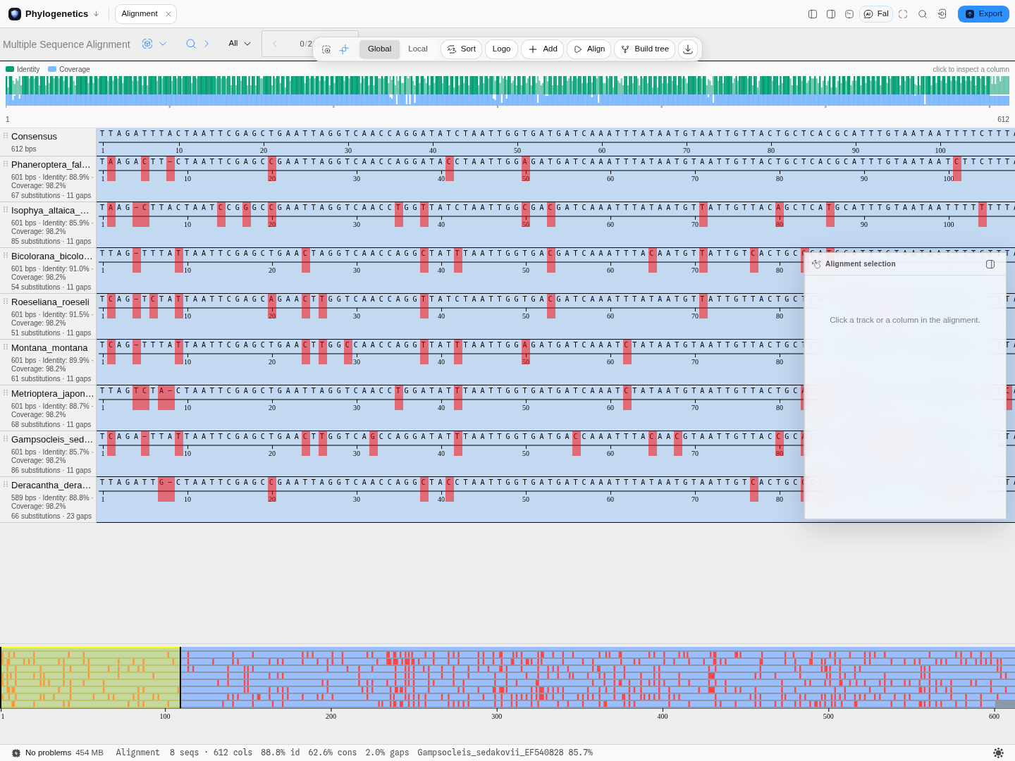
Reading a branch takes three gestures, and each answers a different question. Hover a node or
a tip for its own numbers, without changing anything: Clade of 44 tips · support 86 · branch 0.0121. Click it to select that clade, in the tree and in the alignment beside it. Right-click
for the verbs that act on it: root here, rotate, zoom to the clade, remove the clade, keep only
the clade, copy its tip labels, copy it as Newick.
Zoom and keep only are two different verbs and the difference matters. Zooming shows one clade larger while the tree behind it is untouched: the statistics, the exports and the readings along the bottom of the window all still describe the whole tree, and a banner names how many of the total tips you are looking at and offers the way back. Keep only this clade actually removes the other taxa — a new tree, with its own statistics, revertible but real. Reach for the first when you want a closer look and the second when the other taxa do not belong in the analysis.
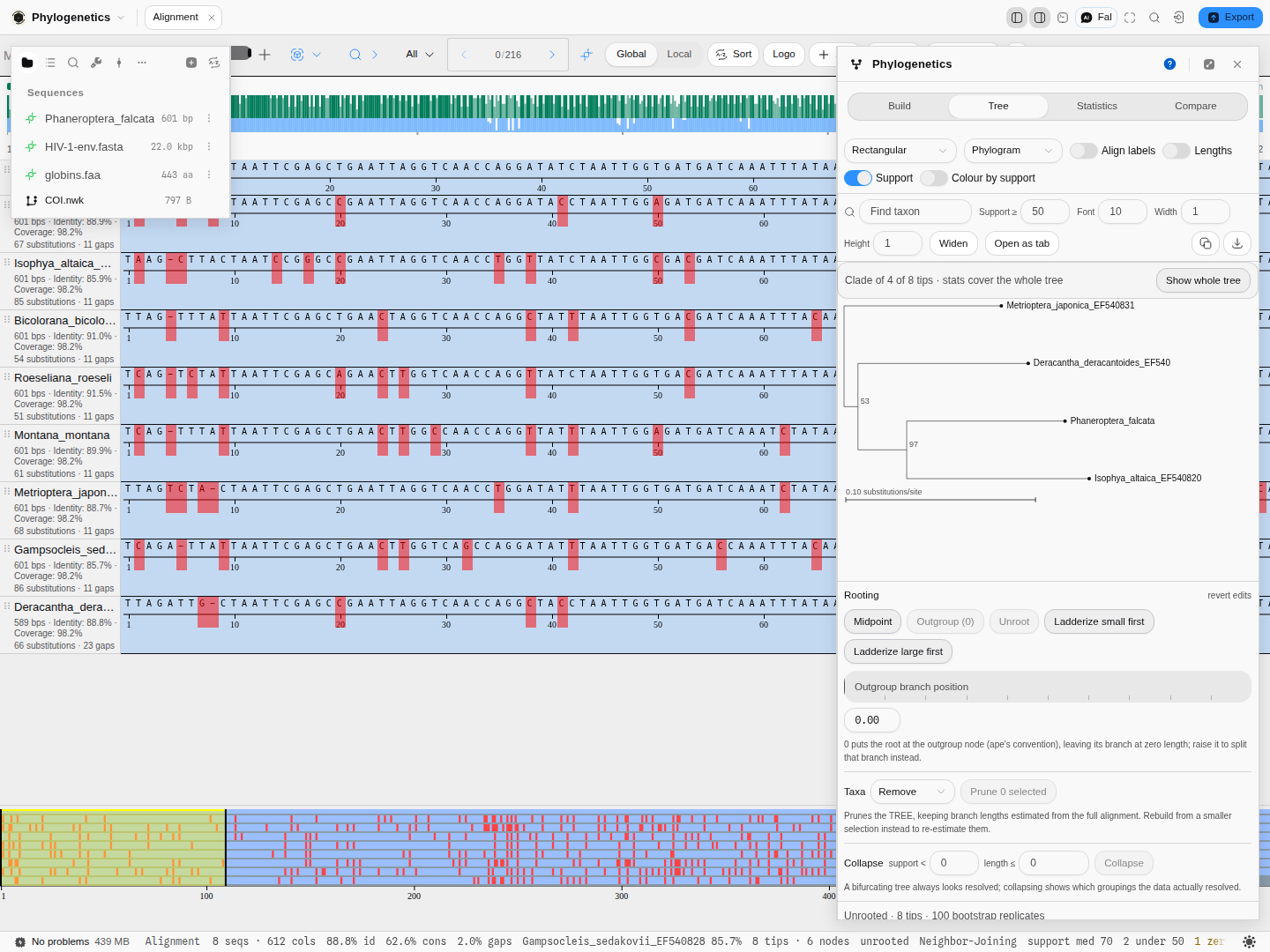
Support is deliberately printed with no unit. A confidence value in a Newick file may be a bootstrap
percentage, a Bayesian posterior probability or an aLRT score, and the file does not record which,
so adding a % would assert something the data does not say. A tip never shows a support value
either, since the only number available there belongs to the branch above it.
The line along the bottom of the window reads the tree, so the numbers that decide whether a drawing can be interpreted at all are visible without opening a tab: how many tips and internal nodes, whether it is rooted, which method inferred it, the median branch support with how many branches fall under 50, how many branches have zero length, and the Pybus-Harvey γ. Those are the facts a bifurcating drawing hides — it looks equally resolved whether the data resolved it or not.
Context flows both ways. Click a clade and those sequences are selected in the project and highlighted in the alignment beside it; select a track in the alignment and its tip highlights in the tree; and the tree's tip order can be pushed back to the alignment as a sort order, so the rows read in the order the tree implies rather than the order the file happened to list them.
Tree files are ordinary project files. .nwk, .newick, .tree, .tre, .dnd, .nex,
.nexus, .nexml and .phyloxml all import, sit in the sidebar next to the alignment they came
from, and survive a reload. A tree that arrived that way is labelled with the file it came from, and
it says plainly that it carries no distance matrix, no substitution model and no bootstrap, so it can
never be mistaken for something inferred here.
The tree drawing follows you down to smaller screens: at 1024 px wide the controls reflow to two rows and the tree, the shape statistics, the lineages-through-time curve and the six-column model-comparison table all stay whole.
On the drawing, all of it a view of the tree rather than a change to it (the statistics and the exports still describe the whole tree):
- The alignment beside the tips: for a tree built here, each sequence is drawn level with its own tip, every column marked where it differs from the majority consensus of the alignment, as a mismatch or a gap. Reading down the strip shows which characters a clade shares, and a tip whose row is crowded with marks against otherwise quiet neighbours is the one to check first for a misaligned or contaminated sequence
- Clade color and collapse: right-click a node to color its clade or draw it as one triangle, from the clade's common ancestor to its deepest tip, named by the genus its tips share. Both are tied to the clade's set of taxa, so they survive rerooting wherever that set is still a clade
- Tip data from the tree file: a NeXML file can say something about each taxon (its NCBI taxon, its rank, its parent taxon). Pick one and it is drawn as a strip of runs beside the tips, or a ring around a circular tree, each run's value printed once. The colors only tell neighbours apart, so a value that comes back further down the strip keeps its first color: that is a group the tree does not keep together. On the primate tree bundled with the app, the parent taxon of Galago matschiei recurs away from the other Galago species. The annotations are read exactly as RNeXML reads them; an NCBI identifier is shown as written, since naming it needs the network
Inputs and outputs
It accepts an alignment — sequences that are all the same length, where column i means the same homologous position in every row. That is the whole requirement, and it is load-bearing.
What it refuses, and why it refuses rather than guessing:
| Input | What you are told |
|---|---|
| Fewer than three sequences | A tree needs at least 3 sequences; this one has 2. Two sequences have exactly one unrooted topology, so there is nothing to infer. |
| Sequences of unequal length | These sequences are not aligned (lengths range 589-601 bp). Build a Multiple Sequence Alignment first. |
| A FASTA pasted into a tree box | This does not look like a tree: it looks like a FASTA file. |
| Any other non-tree text | This does not look like a tree: no NEXUS, PhyloXML or NeXML markup was found, and a Newick tree must end in a semicolon. |
| A NEXUS file with no TREES block | This NEXUS file has no TREES block, so it contains no trees to read (it holds TAXA, CHARACTERS). When it holds a character matrix, the message says to open it as an alignment and build a tree from it. |
The unequal-length refusal is the important one. Distance models are defined per aligned column. Feed raw, un-aligned homologues to a distance model and every calculation still succeeds — it simply compares position 200 of one gene against position 200 of another, which are not the same site. You get a tree, it looks entirely normal, and it is wrong. So the tool will not do it, and it says which lengths it saw.
It produces a tree with branch lengths and, if you asked for bootstrap, support values; the distance matrix it was built from; the shape statistics — tree height, total length, diameter, the branch-length distribution, zero-length branches, cherries, Colless and Sackin imbalance, treeness, the Pybus-Harvey gamma with its P-value, and the clock readouts gamma depends on; and a lineages-through-time curve. A tree file holding several trees (bootstrap replicates, a posterior sample, one tree per line) opens its first tree and names the others, by the name the file gives each tree or by its position, in the tree's notes and in Problems. To summarise all of them, use the consensus on the Compare tab. Export is Newick, NEXUS, PhyloXML or NeXML for the tree, SVG or PNG for the drawing, or Save to project, which writes the tree back as a project file that reopens straight into this tool.
Worked example
The Phylogenetics sample project opens on eight cricket COI genes (mitochondrial cytochrome oxidase I, the standard animal barcoding locus) together with a maximum-likelihood tree of eighteen related sequences, so a tree you build here has something independent to be checked against.
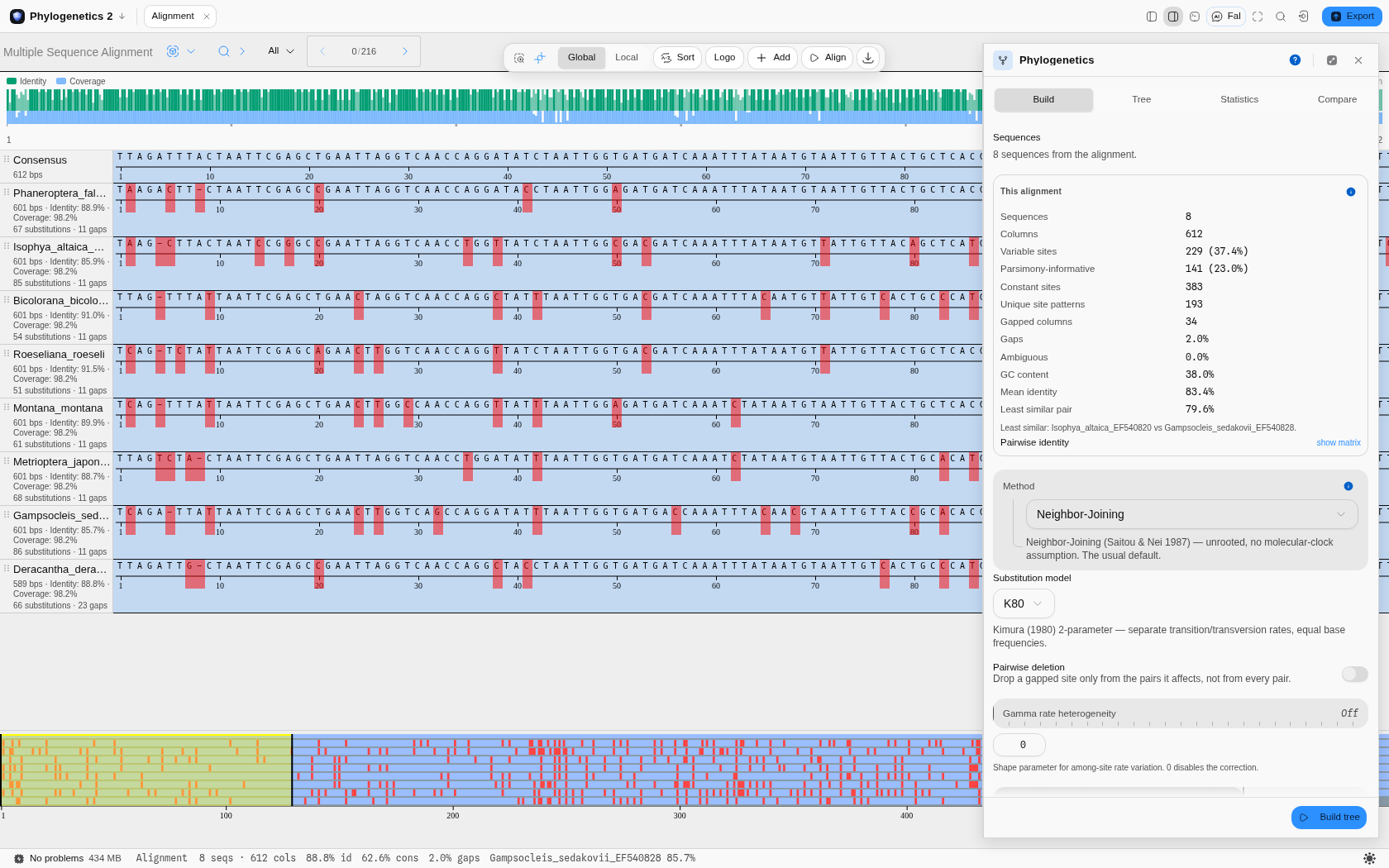
1 · The alignment is diagnosed before you infer anything. The panel's This alignment box reports, for these eight sequences:
| Sequences · columns | 8 · 612 |
| Variable sites | 229 (37.4%) |
| Parsimony-informative | 141 (23.0%) |
| Constant sites | 383 |
| Unique site patterns | 193 |
| Gapped columns · gaps | 34 · 2.0% |
| GC content | 38.0% |
| Mean identity | 83.4% |
| Least similar pair | 79.6% — Isophya altaica vs Gampsocleis sedakovii |
Read this before choosing a method. 141 parsimony-informative sites is the number that matters: those are the only columns that can distinguish one topology from another. The 383 constant sites contribute nothing to the branching order (they do inform branch lengths and the invariant-sites parameter). At 83.4% mean identity these sequences are close enough that model choice will not change the topology much — which is exactly why the project ships a second dataset, 19 divergent HIV-1 env genes, where it does.
2 · Build. Neighbor-Joining under K80, 100 bootstrap replicates. About a second.
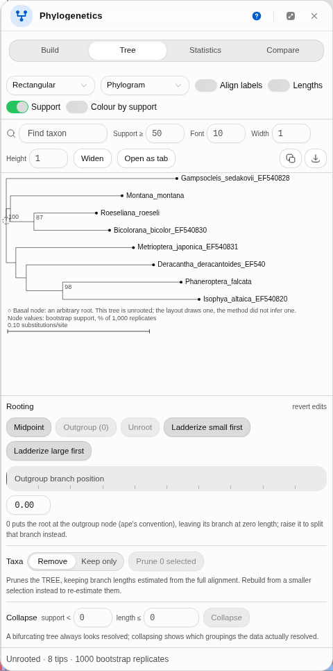
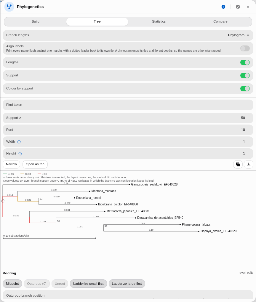
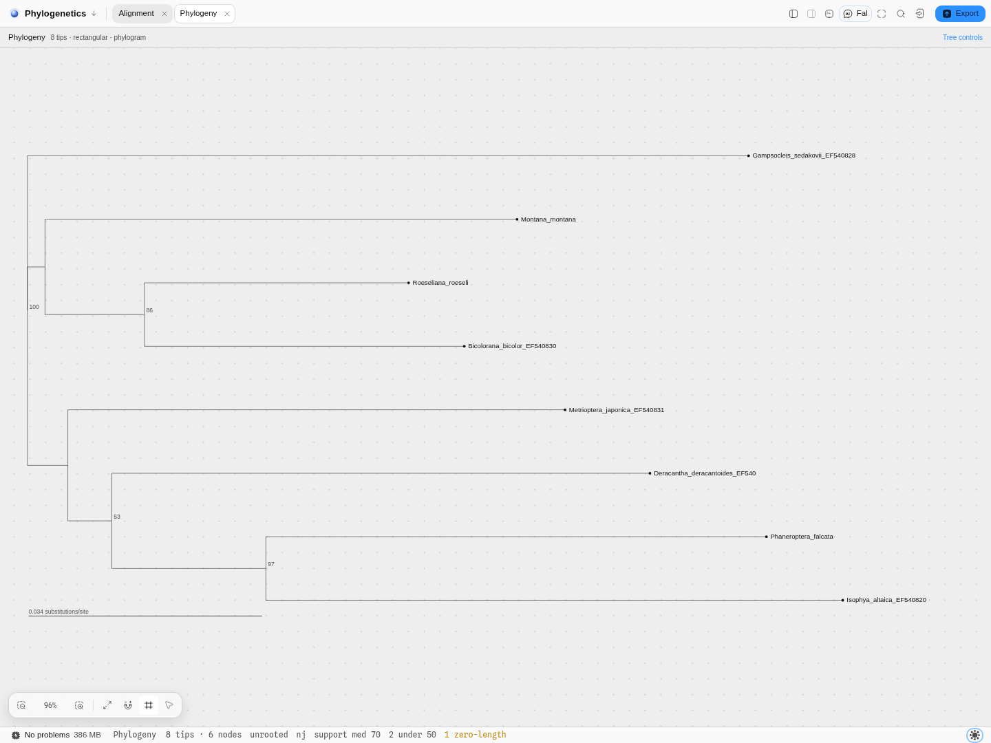
3 · Read the tree. Eight tips, six internal nodes, a scale bar of 0.034 substitutions/site. Support sits on the internal branches: 100 and 97 on two of them, 86 on a third, 53 on a fourth.
4 · Read the support honestly. The Statistics tab summarises it: mean 65.5, median 69.5, lowest 27, highest 100 — and 4 of 6 branches at or above 50, 3 of 6 above 70, 2 of 6 above 95. So two groupings in this tree are solid and the rest are suggestions. A tree drawn without support values would have looked equally confident about all six.
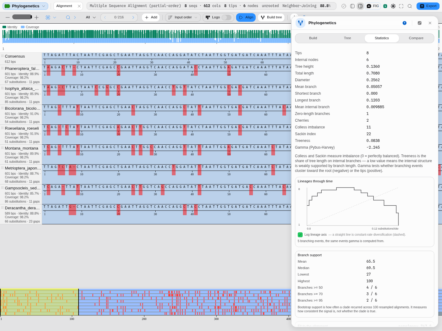
5 · Read the shape. Tree height 0.1408, total length 0.7242, diameter 0.2628, longest branch 0.1219, mean internal branch 0.01035, one zero-length branch, Colless imbalance 11, Sackin index 22, treeness 0.0857, Pybus-Harvey gamma −3.629 (P 0.000284).
Three of those deserve attention. Treeness 0.0857 is the share of total tree length sitting on internal branches — under 10% here, meaning almost all the evolutionary change is on the terminal branches and the internal structure is supported by very little. That is the same fact the modest bootstrap values reported, arriving by a different route. One zero-length branch means the data resolved nothing at all at that node; a bifurcating tree always looks fully resolved, which is what the Collapse control is for.
And gamma comes with the assumption it stands on, which is the third. The Pybus-Harvey gamma reads the intervals between branching events as intervals of TIME, and asks whether they bunch toward the root (negative, an early burst) or toward the tips (positive, a recent radiation), against what a constant-rate birth process predicts. It is a standard normal deviate, so the P-value beside it is the two-tailed test of that constant-rate null — and it is only a statement about diversification on a clock-like (ultrametric) tree, one where every tip sits the same distance from the root.
A tree inferred from sequence divergence is generally not that tree. Rates differ between lineages, so the tips end up at different depths, and the panel says by how much: "Not ultrametric: root-to-tip distances span 54.4% of the deepest tip, or 1.48 mean branches" on this one. Below one mean branch the raggedness cannot reorder any branching event and the panel says so instead — a published time-calibrated tree usually lands there, off by rounding rather than by biology. Above it, part of what gamma is scoring is rate variation rather than diversification, and the same goes for the lineages-through-time curve, which on a non-ultrametric tree falls once the shallowest tips terminate. A real lineage count never falls.
This matters more than a caveat usually does, because the number is not even stable across implementations when the assumption fails: on the cricket COI tree bundled with this tool, three widely used implementations of gamma return −6.12, −2.16 and −3.22 for the same tree, and a fourth declines to answer. To get gamma as a diversification result, give it an ultrametric tree — a time-calibrated phylogeny, or one built under UPGMA/WPGMA, which force the clock (and can recover the wrong topology when the clock is false, as the method list says above).
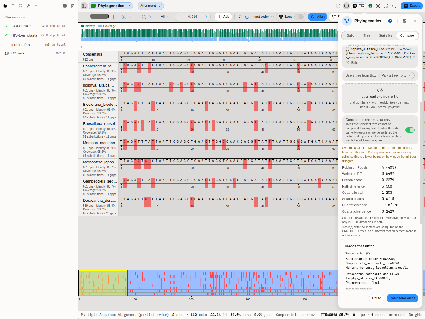
6 · Compare it to a reference tree. Open COI.nwk in the Compare tab. It carries eighteen
taxa where your alignment has eight, which is the usual case when the other tree comes from a paper,
so the comparison names the mismatch — how many taxa each tree has, how many they share, and which
labels only the other one carries — and offers to score them over the eight they have in common.
Every metric below is then reported for those eight, with the disagreeing clades listed by name.
Controls
Every parameter the engine takes is on the panel; none is a hidden default.
Build — method · substitution model · pairwise vs complete deletion · gamma rate heterogeneity (shape parameter, 0 disables) · bootstrap replicate count · and, for maximum likelihood, individual switches for which parameters to estimate (substitution rates, base frequencies, gamma shape, invariant proportion) and whether to search topology · and, for the Bayesian method, the likelihood model (JC69, F81, K80, HKY) and kappa, the number of iterations, the burn-in, the sampling interval, the seed, and the Gamma prior on theta (its mean and shape) with the value the chain starts from. The panel states how many trees the settings will keep before you run.
Tree — layout (rectangular · slanted · circular · unrooted, and for unrooted a choice of two algorithms) · branch transform (phylogram · cladogram · Grafen depth) · align tip labels · branch-length labels · support labels with a threshold · colour-by-support · tip font size · horizontal and vertical stretch · find-a-taxon search.
The same controls by name, as the panel labels them:
Build: distance and support
| Control | Default | What it sets |
|---|---|---|
| Substitution model | K80 | The distance correction |
| Gamma rate heterogeneity | 0 | Shape parameter for among-site rate variation; 0 disables it |
| Branch support | Bootstrap | Bootstrap, or one of the branch tests (aLRT, aBayes, SH-aLRT) |
| Bootstrap replicates | 100 | Resampled alignments, each built into a tree |
| Workers | 3 | How many replicates run at once. Same replicates and same support, whatever the count |
| RELL replicates | 10,000 | For SH-aLRT: resamples the per-site log-likelihoods, not the alignment, so no tree is re-inferred. PhyML uses 10,000 |
| Midpoint root | off | Distance methods return an unrooted tree; this roots it at its midpoint |
Build: maximum likelihood
| Control | Default | What it sets |
|---|---|---|
| Likelihood model | K80 | The substitution model the likelihood is computed under |
| Gamma rate categories | 1 | 1 disables rate heterogeneity; 4 is the usual choice |
| Gamma shape (alpha) | 1 | Lower means more rate variation between sites. The starting value when the shape is estimated |
| Invariant sites | 0 | The proportion of sites that never change. The starting value when it is estimated |
| Topology search | Nearest-neighbor interchange | Or NNI, then prune-and-regraft; or NNI, then prune-and-regraft, then bisect-and-reconnect. Each step searches wider and costs more |
Build: Bayesian
| Control | Default | What it sets |
|---|---|---|
| Kappa | 2 | The transition/transversion ratio, fixed for the run unless sampled |
| Sample kappa · Sample base frequencies · Sample Gamma shape | off | Let the chain sample each instead of holding it fixed |
| Rate categories (+Γ) · Gamma shape | 1 · 1 | Among-site rate variation, as for maximum likelihood |
| Clock | Strict | Strict, Relaxed (uncorrelated lognormal), or None (unrooted, free branch lengths) |
| Branch-length prior rate | 10 | Each branch length is exponential with this rate a priori. MrBayes uses 10 |
| Rate spread start (sigma) | 0.1 | Where the relaxed clock's log-scale spread of branch rates starts. It is sampled |
| Iterations | 20,000 | Length of each chain |
| Burn-in | 5,000 iterations | Discarded from the start of each chain |
| Sample every | 100 iterations | The thinning interval |
| Independent runs | 1 | Two or more runs are pooled and compared, so the split-frequency deviation and PSRF can say whether they found the same posterior |
| Minimum split frequency | 0.1 | A clade enters the split-frequency deviation only if some run sampled it this often. MrBayes uses 0.10 |
| Heating temperature | 0.1 | Flattens the heated chains; higher means fewer successful swaps. MrBayes uses 0.1 |
| Theta prior mean · Theta prior shape | 0.036 · 2 | The Gamma prior on θ = 4Nμ for the species-tree model. PhyloNet's default mean is 0.036 |
| Starting theta | 0.02 | Where the chain starts θ. A run whose answer moves with it has not converged |
Tree
| Control | Default | What it sets |
|---|---|---|
| Layout | Rectangular | Rectangular, slanted, circular or unrooted |
| Unrooted method | Equal angle | The unrooted drawing algorithm |
| Align labels | off | Lines every tip label up in one column |
| Lengths | off | Prints each branch's length on it |
| Support ≥ | 50 | Support values below this are not printed |
| Color by support | off | Shades each branch by its support |
| Font · Width · Height | 10 · 1 · 1 | Tip font size and the horizontal and vertical stretch |
| Find taxon | empty | Highlights matching tips |
| Outgroup branch position | 0 | Where on the outgroup's branch the root sits when you reroot |
| Use a tree from this project | — | Opens a tree file already in the project, listed with its tip count |
Stats
| Control | Default | What it sets |
|---|---|---|
| Weight transitions below transversions | on | Transitions are chemically far more frequent, so scoring them equally overstates the change a topology needs |
While it runs: what the panel is telling you
The slow methods say where they are, and the readout is worth reading rather than watching.
A likelihood fit names the stage it is in, and the stages are the algorithm rather than a loading animation. It alternates branch lengths → model parameters → branch lengths again, and only then rearrangements if topology search is on. That order is not arbitrary: branch lengths are fitted first because a starting tree from Neighbor-Joining has lengths on a completely different scale from the model's, and fitting a shape parameter against badly scaled branches sends it to a boundary it then has to climb back from. Seeing Model parameters come round a second and third time is the fit converging, not repeating itself.
Beside the stage is the log-likelihood as it stands — the quantity being maximised. It is the number to watch, because a progress bar can only tell you how many steps are left, never whether the steps are still buying anything. A fit whose log L has stopped moving in the third decimal across two rounds has converged, whatever the bar says.
Model selection counts fits and names the model in each one (Fitting F81+G4+I, 7 / 24), so a sweep that stalls tells you which candidate is the expensive one. A bootstrap counts replicates, and that count is the honest measure of what you asked for: 100 replicates under maximum likelihood is 100 full optimisations, and under parsimony with SPR it is 100 full searches. Both are minutes, not seconds, and the counter is what makes the difference between "slow" and "hung" visible.
Stop really stops. Every long run happens off the main thread, so the editor stays usable while it goes, and stopping terminates the work rather than setting a flag that gets read after the work finishes. Nothing is left half-applied: a stopped run leaves the tree you had.
Align tip labels is worth knowing about before you present a tree. A phylogram ends its tips at different depths, so the names come out ragged and comparing two taxa means tracking a name back across the drawing to find which branch it belongs to. Turning it on prints every name flush against one margin with a dotted leader back to its own tip: the same tree, read in half the time. It applies to the rectangular, slanted and circular layouts. The unrooted layout does not offer it, and that is geometry rather than an omission — an equal-angle drawing radiates in every direction from an arbitrary centre, so there is no margin for the names to be flush against.
How the branches get their length: three transforms
The same tree can be drawn three ways, and the choice is a scientific one rather than a matter of taste, because each answers a different question.
Phylogram — the drawn branch is the inferred branch, so horizontal distance is evolutionary distance and the scale bar means what it says. This is the drawing you read when you care how far apart two taxa actually are. It is the default and it should be, but it has a known weakness: a clade whose branches are all short is squashed into a sliver, and its topology becomes unreadable exactly where the resolution is most in doubt.
Cladogram — every branch counts one, so the drawing shows the shape of the tree and nothing else. Reach for it when the branch lengths are uninformative or when you want to compare topologies between two trees without their lengths distracting you. It draws no scale bar, because there is no scale; the panel says so on the drawing rather than leaving a bar that would be a lie.
Grafen depth — Grafen's (1989) transform. Each node is given a height equal to the number of tips beneath it minus one, those heights are scaled so the root is exactly 1, and each is then raised to a power you choose. Every branch is the difference between its two endpoints' heights, so every root-to-tip path sums to 1 and the drawing is ultrametric by construction — all tips flush at one depth, like a chronogram, but derived from the topology alone.
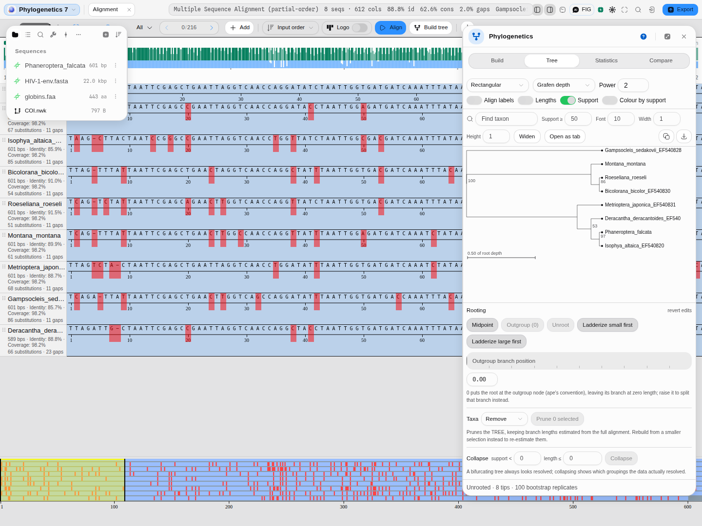
Grafen is the one that surprises people, so it is worth being explicit about what it does and does not tell you:
- It ignores the branch lengths you inferred. A tree with wildly uneven branches gives exactly the same picture as the bare topology. That is the point: it is a way of looking at the balance of a tree without any distance signal in the way, and it is why the same transform is used as a branch-length assignment in comparative methods when a tree has topology but no lengths.
- The power (Grafen's rho) is the knob. Below 1 pushes internal nodes towards the tips, which spreads out the recent splits; above 1 pushes them towards the root, which spreads out the deep ones. At exactly 1 the depth is linear in the scaled tip count.
- The scale bar changes with it. Under Grafen it reads "of root depth", not substitutions per site, because that is the unit the drawing is actually in.
Not offered: a time-calibrated transform. Turning a tree into a chronogram needs calibration points and a clock model, which is a different analysis from anything on this panel — Grafen's ultrametric drawing looks like a chronogram and is emphatically not one, and calling it one would be the mistake this note exists to prevent.
Drawing a tree with no root: two algorithms, not one
An unrooted tree has no root to measure depth from, so the drawing has to choose directions for itself. Two published algorithms do that, and neither replaces the other.
Equal angle (Felsenstein) gives each subtree a wedge of the circle proportional to how many tips it holds, then places every node along the bisector of its own wedge at its branch length. One pass, fast, and it can never produce crossing edges. Its weakness is what the wedges are allocated by: tip count, while the drawing is then filled by branch length, so on an unbalanced tree whole clades end up bunched into a narrow sliver.
Equal daylight (Felsenstein, Inferring Phylogenies, pp. 582–584) starts from the equal-angle drawing and then repeatedly visits each interior node, swinging its subtrees so that the arcs of blank "daylight" between them come out equal. It spreads the tips out, and it costs more: it is iterative, and on a very large unbalanced tree it can produce crossing edges, which equal angle cannot. It only ever rotates subtrees about their own nodes, so every branch length survives it exactly and the scale bar is as true of a daylight drawing as of an equal-angle one.
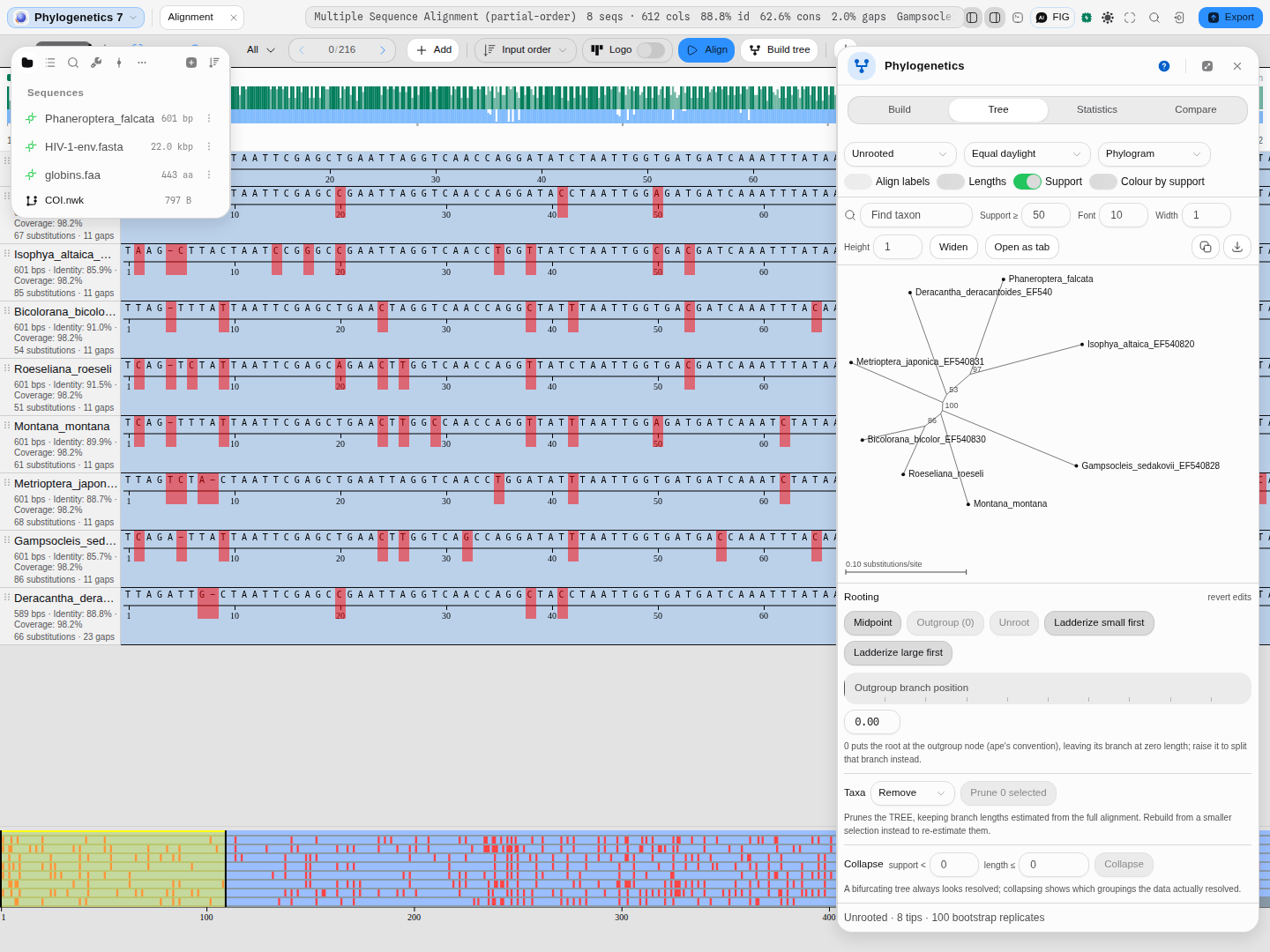
Which to use: start with equal angle. Switch to daylight when the tree is unbalanced enough that tips are colliding — that is the case it was invented for, and on a well-balanced tree it will barely move anything.
Rooting and editing — midpoint rooting · outgroup rooting with an adjustable branch position · unroot · ladderize small-first or large-first · prune or keep selected taxa · collapse branches below a support or length threshold · rotate at a node. Every edit is revertible to the tree as built.
Ladderizing sorts each node's children by how many tips are under them, so the ladder runs consistently down or up the page instead of the branches sitting in whatever order the method emitted. Both directions are offered because which one reads better depends on where the group you care about sits: the convention in most published figures is the large clades first, but if your outgroup is a single tip you will usually want it at one end rather than buried.
Compare — another tree by paste or file · replicate trees for a consensus, strict or majority-rule at an adjustable cutoff · the distance matrix · the input-versus-patristic table.
Both boxes read any tree format — Newick, NEXUS, NeXML or PhyloXML — and the replicate box takes either one file holding several trees or one tree per line. A multi-tree Newick file is accepted however its trees are broken across lines, because the semicolon ends a tree and the line breaks carry no meaning; that is the rule the format actually specifies, and files written by other programs rely on it. Paste something that is not a tree and it says so, naming what it looks like instead.
Two controls exist specifically to stop the tool overclaiming. Pairwise deletion decides whether a gapped site is dropped from every comparison or only from the pairs it affects, which changes every distance in the matrix. Collapse turns branches the data did not resolve into polytomies, because a bifurcating drawing asserts a resolution that a zero-length branch does not have.
Algorithms you can choose
Nine inference methods, in four families answering four different questions.
| Method | What it does | Assumes a clock |
|---|---|---|
| Neighbor-Joining (Saitou & Nei 1987) | Agglomerates the pair minimising total tree length. The usual default. | No |
| BIONJ (Gascuel 1997) | NJ weighted by the variance of each distance — better when distances are large. | No |
| FastME balanced (Desper & Gascuel 2002) | Minimum evolution: stepwise insertion then NNI/SPR topology search. | No |
| FastME OLS | The same, under ordinary least squares rather than balanced weighting. | No |
| UPGMA | Averages distances weighted by cluster size. Produces an ultrametric tree. | Yes |
| WPGMA | The same without size weighting. | Yes |
| Maximum Parsimony | Minimises total character changes; no substitution model at all. Susceptible to long-branch attraction. Searches by NNI, by NNI then SPR, or by NNI then SPR then TBR. | No |
| Maximum Likelihood | Optimises branch lengths, and optionally the model and topology, to maximise the probability of the alignment. Searches by NNI, by NNI then SPR, or by NNI then SPR then TBR — the same choice parsimony offers, and for the same reason. | No |
| Bayesian (MCMC) (Wen & Nakhleh 2018, one population) | Metropolis–Hastings sampling of the tree's topology (nearest-neighbour interchange), its node heights and theta, under JC69, F81, K80 or HKY, optionally +Γ, with the parameters held fixed or sampled, a strict or uncorrelated lognormal relaxed clock with a constant-size coalescent prior on the tree, or no clock (unrooted, Exponential branch lengths). Reports clade posterior probabilities on the majority-rule consensus. | Yes |
Both parsimony and likelihood offer three topology searches, and the choice changes the answer. All three hill-climb from the Neighbor-Joining tree and all three return a local optimum; they differ in how far they can see, and they are steps up rather than alternatives — each runs the cheaper moves first, because every NNI move is also an SPR move and every SPR move is also a TBR move.
NNI only swaps neighbouring branches. SPR can cut a whole clade out and graft it anywhere else, which lets it leave an optimum NNI cannot — under likelihood as well as under parsimony: on this app's cricket sample, a likelihood search by NNI alone stops 0.25 log-likelihood units below the one that then sweeps SPR, from the same starting tree. On this app's own sample data SPR finds the shorter tree in both cases: 974 steps against 975 on 18 cricket COI barcodes, and 2,133 against 2,161 on 25 HIV-1 env genes.
TBR cuts a branch in two and rejoins the halves by any pair of their branches, which also lets it turn the detached half around before reattaching it — the one thing prune-and-regraft cannot do. It is the widest search here, and the cost is worth stating as a count rather than an adjective: on those same 18 cricket barcodes it considers 1,874 distinct trees per sweep against 842 for prune-and-regraft. That is 2.2 times the candidates, but only about 1.4 to 1.7 times the wall clock — measured end to end from 8 to 14 taxa, because the rearrangement sweep is one stage of a fit rather than the whole of it. Under parsimony the gap is wider, because each TBR candidate is scored whole where prune-and-regraft scores them incrementally.
It pays when a search has stopped somewhere you do not believe. On the first ten of those cricket barcodes, from a deliberately poor starting tree, prune-and-regraft stalls at 598 steps and TBR reaches 594 — four steps that no amount of NNI or SPR from that start will find. A run that accepts no TBR move has told you something too, namely that your tree is not merely NNI-optimal.
All of this compounds with resampling: because a bootstrap re-runs the whole search on every replicate, SPR at 100 replicates is 100 searches and TBR at 100 replicates is 100 wider ones, which the panel warns about rather than letting it look hung.
The clock column is not decoration. UPGMA and WPGMA force every tip to be equidistant from the root, which is only correct if all lineages evolve at the same rate. When they do not, UPGMA does not merely lose accuracy — it can recover the wrong topology. The tool states this assumption next to each method rather than in a footnote.
Fourteen distance models, from uncorrected p-distance up: raw · N · transitions only · transversions only · JC69 · K80 · F81 · K81 · F84 · T92 · TN93 · Log-Det · indel · indel-block, each optionally with a gamma rate correction. The awkward ones are worth knowing: Log-Det is the one to reach for when base composition differs between lineages, which breaks every model that assumes stationarity; T92 corrects for G+C bias specifically; and raw saturates at large distances, which is why a correction exists at all.
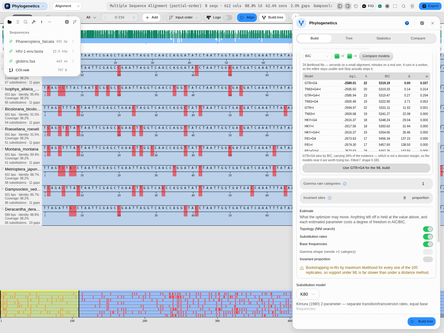
Six models for maximum likelihood — JC69 · F81 · K80 · HKY · TN93 · GTR — each with optional discrete-gamma rate categories and a proportion of invariant sites. Compare models fits every combination on one shared topology and ranks them by AIC, AICc or BIC with Akaike weights. It fits them all on the same topology deliberately, and refuses to search topology per candidate rather than quietly defaulting that off: comparing models that were each allowed to pick a different tree compares two things at once.
Every candidate is fitted once, and each keeps all three scores, so changing the criterion after a run re-ranks the table you already have instead of re-fitting anything. That is not just a speed convenience: it means you can look at the same 24 fits under AIC, AICc and BIC in a few seconds and see for yourself whether the choice of criterion changes the answer, which is the question worth asking. On the eight cricket COI genes the sweep takes about a minute and a half and the winner is the same under both AIC and BIC — but carrying only 0.34 of the Akaike weight, which the panel says out loud rather than presenting a winner as if it were settled. Weights are the honest reading of a ranking: a model that holds a third of the evidence has three-in-ten rivals worth trying.
Five tree-to-tree metrics, because "how different are these trees" is not one question: Robinson-Foulds counts clades present in one and not the other; weighted RF and the branch score (Kuhner & Felsenstein 1994) take branch lengths into account; path difference (Steel & Penny 1993) and quadratic path difference compare every pairwise path; and the quartet distance reports the full Estabrook (1985) breakdown of which four-taxon relationships agree, disagree or are unresolved. Two trees can be identical by one and far apart by another.
Every one of them is defined only over a single taxon set, and that is a property of the mathematics rather than a limitation here: a clade is a partition of the taxa, so two trees that do not contain the same taxa have no partitions to compare. Trees from different studies almost never match — one includes an outgroup you did not sequence, another has three species you do not. The honest answer is to compare them over what they share, which means pruning both to the common set first and saying so. Read such a number as a lower bound. Removing a taxon can merge two clades into one or delete a clade entirely; it can never create a disagreement that was not already there. So the trees may differ more than the pruned comparison shows, and never less. Below four shared taxa there is nothing to compare at all: an unrooted tree of three or fewer tips has no internal branch, so every metric would read zero for want of anything to disagree about.
The science
Distance methods compute a pairwise distance matrix under a substitution model and then build a tree that best represents it. Fast, and the accuracy ceiling is set by the matrix: any information the pairwise distances discard cannot be recovered later.
Parsimony ignores models entirely and looks for the tree needing the fewest character changes. Its known failure mode is long-branch attraction: two rapidly-evolving lineages accumulate independent changes that happen to coincide, and parsimony reads that coincidence as shared ancestry. The consistency and retention indices reported alongside the score are how you notice.
Maximum likelihood asks which tree makes the observed alignment most probable under an explicit model, computed by Felsenstein's pruning algorithm. It is the slowest and the only one that returns a likelihood, which is what makes AIC and BIC available and therefore what makes model selection possible at all.
Rate heterogeneity matters more than model choice usually does. Real sites do not evolve at one rate: third codon positions turn over far faster than first and second. Discrete-gamma categories (Yang 1994) let a model express that, and a proportion of invariant sites accounts for positions that cannot change at all. Adding gamma to a simple model typically improves fit more than swapping the simple model for a complicated one.
Bootstrap support resamples the alignment's columns with replacement, rebuilds the tree from each replicate, and reports how often each clade recurred. Under maximum likelihood the replicates are re-fitted by maximum likelihood, not by a faster distance method — support must measure the estimator that produced the tree. Read the number correctly: it measures how consistent the signal in your data is, not whether the clade is true. A systematically biased alignment produces high support for the wrong tree.
Provenance of correctness. Every engine here is checked against the established
implementations by the same input: distances against ape's dist.dna over 180 cases; BIONJ and
FastME against ape over 60 runs, each pinning the edge matrix, edge order, branch lengths and tip
numbering; parsimony and consensus against Biopython; Robinson-Foulds, weighted RF, branch score and
path difference against phangorn; the quartet breakdown against the R Quartet package;
site statistics against ape's seg.sites; rate matrices and transition probabilities against
phangorn over 126 cases; likelihoods against phangorn's pml for both total and per-site
values; and model selection against the real phangorn::modelTest, candidate for candidate. On that last
one the honest detail is worth stating: across 24 candidates the degrees of freedom agree exactly,
the selected model agrees under both AIC and BIC, and the top-five ranking agrees — but the
log-likelihoods themselves differ by up to a few units on the models with free base frequencies,
in both directions, because two optimisers stop at slightly different points on a flat surface.
The ranking is what model selection uses, and the ranking agrees.
The Bayesian sampler is checked twice, because a sampler has no single right output. Its
deterministic parts (the starting tree, the likelihood, the coalescent density, the prior and the
trace statistics) are checked value for value against PhyloNet's MCMC_SEQ sampler as
re-implemented in PhyNetPy. Its output is checked as a distribution. First, on data that carry no
information, it must sample the fifteen rooted four-taxon topologies at the coalescent's own odds:
two ranked histories for each balanced tree and one for each caterpillar, out of eighteen. Second,
its clade posteriors on the cricket barcodes must agree with four independent reference chains.
The no-clock model is checked against MrBayes: its split posteriors and tree length must land on
MrBayes' under the same priors. The relaxed clock is checked against BEAST 2.7: on the cricket barcodes its clade posteriors, root
height and clock sigma must land on BEAST's under the same model and priors.
Where the reference implementations disagree with each other or contain a genuine error, the difference is documented rather than inherited. Two worth knowing as a user:
- Biopython's
upgmais actually WPGMA — it averages distances without weighting by cluster size. Both are offered here under their correct names, so if you are reproducing a published tree built with Biopython's "UPGMA", the method you want here is WPGMA. - Bootstrap support survives export. Support written into the same slot as an internal node's
name is a well-known way for it to vanish or to reappear as a clade named
Inner187.00; here the slot goes to the confidence, asape, RAxML, IQ-TREE and FigTree all do.
Limitations
- The Bayesian method is a one-population model, with or without a clock. With no clock the
tree is unrooted, every branch length is free under an Exponential prior (rate 10 by default, as
MrBayes' unconstrained model), every topology is equally likely a priori, and there is no
coalescent; root it on an outgroup to read direction. With a clock, by default every lineage
evolves at one rate (a strict clock); the relaxed clock is the uncorrelated lognormal (Drummond et al.
2006, as BEAST's
UCRelaxedClockModel): each branch draws its own rate from a lognormal of mean 1 whose sigma the chain samples under an Exponential prior of mean 1/3. The tree is still rooted by the clock, and its branch lengths are times in substitutions per site at the mean rate. The tree prior is a single constant-size coalescent, and the substitution model's parameters (kappa, base frequencies and, with +Γ, the Gamma shape) are held at the values given unless you ask the chain to sample them, under MrBayes' default priors: an Exponential(1) on the shape, a uniform prior on kappa/(1+kappa), and a flat Dirichlet on the frequencies. A sampled parameter is reported with its posterior mean, 95% HPD interval and ESS. Among-site rate variation is discrete-Gamma categories (each category its bin mean, as MrBayes and phangorn compute it). There is no autocorrelated clock, no random local clock and no species tree. A clade's posterior probability is conditional on all of that, and when rates differ between lineages the clock pulls the tree towards the wrong root and can move clades. - Heated chains help, they do not guarantee. With more than one chain per run (Metropolis-coupled MCMC, as MrBayes runs it), chain j samples the posterior raised to the power 1/(1 + temperature × j), one random pair of chains tries to swap states every iteration, and only the cold chain is kept. The Statistics tab shows how often each pair swapped; a pair that almost never swaps is not helping, so lower the temperature. A valley deep enough can still trap every chain, which is why independent runs and their convergence diagnostics are still worth running.
- Bayesian support is not a fifth support column. Bootstrap, aLRT, aBayes and SH-aLRT measure a branch on a tree you already have; the Bayesian method infers the tree, and its numbers are the posterior probabilities of the clades it sampled.
- A long fit reports no progress, only cancellation. Everything heavy runs off the main thread and Stop genuinely stops it, but there is no percentage while it runs.
- Maximum likelihood gets expensive quickly. Measured on 600 bp with GTR and all parameters estimated: about 0.9 s for 6 taxa without topology search and 2 s with it; 3.6 s and 12 s at 8 taxa; 8.6 s and 62 s at 12. The panel warns above 8 taxa and names topology search as the expensive knob.
- The quartet distance is capped by taxon count, because it enumerates every four-taxon subset. Above the cap the metric is omitted rather than left to hang.