
Digital PCR
Turn partition counts into an absolute concentration.
| Reached by | Tools → Digital PCR (dPCR) |
| Sample project | qPCR & digital PCR |
What it does
Digital PCR does not measure a signal and compare it to something. It splits your reaction into thousands of tiny partitions, amplifies each one separately, and counts how many came out positive. That count is the measurement — no standard curve, no reference gene, no calibrator.
The arithmetic has one subtlety, and it is the whole method. You cannot simply say "3,474 positives out of 26,446 partitions means 3,474 molecules", because a partition that received two molecules looks exactly like one that received one. So the concentration is recovered from the partitions that came out negative, which can only mean they received nothing:
λ = −ln(1 − k/n) copies per partition
At low occupancy the correction is small. At high occupancy it is everything: at 94 % positive, the naive count understates the true concentration roughly three-fold. λ divided by the partition volume is copies per microlitre of reaction, and multiplying back through your dilution chain gives the concentration of the sample you started from.
Because the answer is a count, the uncertainty is a counting uncertainty — a binomial confidence interval on k/n, carried through the same logarithm. Which interval you use is your choice here, not a hidden default, and at the extremes the choice moves the answer.
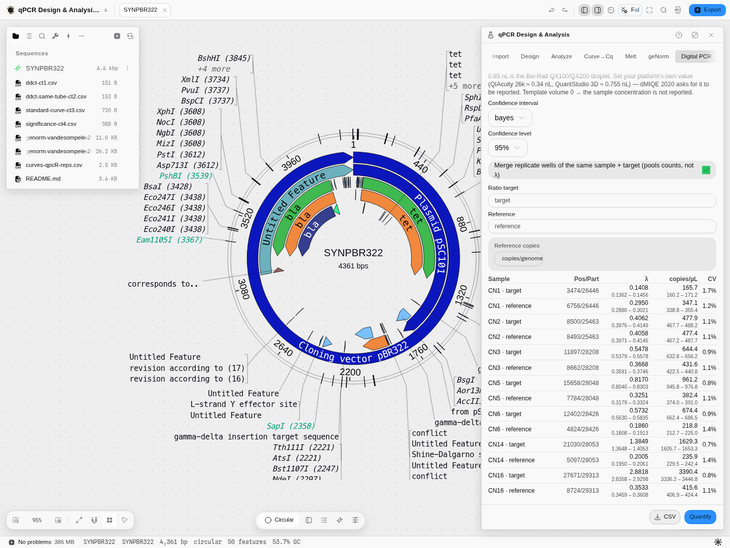
A real 28-well Bio-Rad QX100 copy-number run: seven samples, each with a target and a reference assay, quantified to copies per microlitre with an interval on every row.
What this computes
Per well, from the partition counts
- λ, the mean number of template copies per partition, as −ln(1 − k/n) — the Poisson correction that turns a positive fraction into a concentration
- a confidence interval on λ by any of eleven methods on the binomial scale — exact (Clopper–Pearson), Wilson, Agresti–Coull, Wald with and without continuity correction, logit, Jeffreys, Bayesian, likelihood-ratio, profile-deviance and the arcsine transform. Which one you pick is stated with the answer, because near 0 and near 1 they disagree
- partition occupancy (k/n), the quantity dMIQE 2020 asks to be reported and the one that decides whether the Poisson estimate is still informative — above roughly 90 % occupied, λ is compressed
- copies per µL of reaction, copies per reaction and copies per µL of original sample, each derived only when the volume it needs was supplied and omitted rather than defaulted when not
- precision: the delta-method coefficient of variation, the relative interval width, and a flag when the delta method is outside the range where it is reliable
When partitions are not all the same size
- a volume-variance correction (Poisson-Plus), because the standard estimator assumes every partition holds the same volume and a real chip or emulsion fills to a distribution. The negative fraction is an exponential function of volume, so a spread biases the concentration downward — hard at high occupancy, and hardly at all at low. Two forms are offered and they answer the same question with different exactness: a normal approximation in closed form, and the exact truncated-normal result, which is the honest density because a partition cannot hold a negative volume. Both reduce to the standard estimate when the spread is zero
- the size of the correction, always, beside the uncorrected number. A corrected concentration is not comparable with an uncorrected one, so the reading says which it is and by how much they differ
- the correction runs only when you state a spread. There is no universal value: the coefficient of variation of partition volume is a property of the platform and, for at least one instrument, is re-estimated per chip from that chip's own passive-reference signal. One published figure is offered by name with its citation — 754.72 pL at a 3.03 % CV, measured over 96 QuantStudio 3D chips — and nothing is applied until you choose it
Across wells
- replicate pooling that sums counts rather than averaging λ — averaging the transformed value is a different and wrong estimator
- the exact Poisson rate ratio between two assays of the same sample, with its confidence interval and p-value, and the copy number that follows from a stated reference ploidy
- quality checks that name the well and the reason, never a colour alone
When you'd use this
- You need an absolute number, not a ratio. Viral load, GMO content, a spike-in, a library concentration before sequencing — anything you have to report in copies rather than in fold change.
- Your target is rare. Counting a handful of positive partitions out of twenty thousand is a more honest measurement than reading a Cq at cycle 38.
- You are measuring copy number. Run the target and a known two-copy reference in the same reaction, and the ratio of their concentrations is the copy number — with an exact test behind it rather than a ΔΔCt approximation.
If your instrument reports Cq values rather than partition counts, you want qPCR Design & Analysis instead. To put an interval on something you compute from these numbers — a ratio, a dilution chain, a normalised concentration — take them to the Uncertainty tab of that same panel.
Where it lives
Tools → Digital PCR (dPCR) opens the qPCR panel on its Digital PCR tab. It works on counts rather than on the sequence you have open, so it neither needs nor touches the document on the stage.
Inputs and outputs
In: a well table with, at minimum, the number of positive partitions and the number of valid
partitions per well. Sample and target names are optional but let the tool pool replicates and pair
assays for a copy-number read. Instruments name these columns differently and the tool accepts the
real names as well as its own — Bio-Rad's AcceptedDroplets and QIAcuity's Valid partitions both
work, comma- or tab-separated, so a spreadsheet paste is enough. Partition counts also come straight
out of an RDML file through the Import tab.
Out: per sample — λ with its confidence interval, copies per microlitre of reaction, copies per microlitre of the original sample once you enter the dilution chain, and a precision CV. Plus a copy-number table when you name a target and a reference assay.
Both tables export, as two CSVs rather than one, and the split is the grain rather than tidiness: quantification is one row per sample and assay, while a ratio is one row per sample over a pair of assays. Folding them together would write each grain once per the other and leave you a join to undo. The quantification file carries positives out of partitions, λ and copies/µL each with their interval, the CV, and the quality codes behind any flag; the ratio file carries the rate ratio with its interval and p-value, the reference ploidy you set, and the copy number with bounds.
What it refuses, and says so. A negative partition volume, a dilution factor of zero, a table with no partition column — each is named before the run rather than after it. Two results are returned as facts rather than as numbers, because pretending otherwise would be worse: when every partition is positive the negative fraction is zero and λ is infinite, so the tool says the sample is above the assay's dynamic range and asks you to dilute; and when a chosen interval method puts the upper bound above 1, the bound is reported as not computable, naming the methods that will work there instead.
Step by step
1. Open the sample and load a real run
Open the qPCR & digital PCR sample project, then Tools → Digital PCR and press Load example. That brings in a real Bio-Rad QX100 copy-number experiment — 28 wells, seven samples, each with a target and a reference assay in four replicate wells.
2. Tell it about your platform, before you quantify
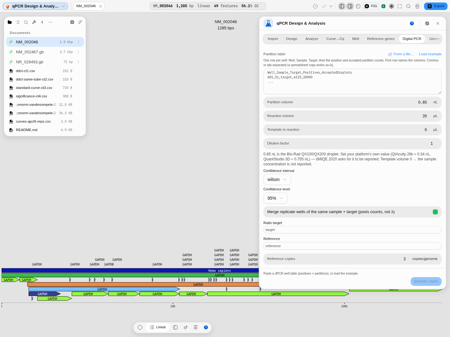
Partition volume is not a cosmetic setting — it is the unit conversion. λ is copies per partition; dividing by the partition volume is what makes it copies per microlitre. The field defaults to 0.85 nL, the QX100/QX200 droplet, and the hint under it names the other common values (QIAcuity 26k ≈ 0.34 nL, QuantStudio 3D ≈ 0.755 nL). dMIQE 2020 asks you to report this number, so set it to yours.
Leave Template in reaction at 0 if you only want the concentration in the reaction; fill it in, with the dilution factor, to get back to the concentration of the sample you started from.
3. Choose the interval, then quantify
Set Confidence interval — ten methods, and at the extremes the choice moves the answer — then press Quantify.
Fourteen rows of λ, one per sample-and-assay, then the ratio table. Every row carries its own interval; nothing here is a bare point estimate.
4. Check the run against itself
The sample names state the expected copy number, so this run is its own control:
| Sample | Ratio | Copy number | 95 % interval |
|---|---|---|---|
| CN1 | 0.514 | 0.95 | 0.92 – 0.99 |
| CN2 | 1.001 | 2.00 | 1.94 – 2.06 |
| CN3 | 1.373 | 2.99 | 2.90 – 3.07 |
| CN5 | 2.012 | 5.03 | 4.89 – 5.17 |
| CN6 | 2.571 | 6.16 | 5.96 – 6.37 |
| CN14 | 4.126 | 13.81 | 13.40 – 14.25 |
| CN16 | 3.172 | 16.32 | 15.93 – 16.72 |
Seven samples, seven copy numbers recovered to two decimal places, with nothing fitted to them.
5. See where the interval choice actually matters
Change Confidence interval from wilson to asymptotic and quantify again. Nothing visibly
moves in the first row — and that is correct, not broken. Then look at CN16 · target (27,671 of
29,313 partitions, 94.4 % occupancy), where the same switch moves the λ interval.
Pick the input where the methods differ, or you will conclude a working control is dead. The
methods separate at the extremes — a handful of positives, or a nearly saturated plate — and agree
to four decimals in the comfortable middle. Switching from wilson to bayes on this run moves the
reported CN16 copy number from 16.32 to 16.31: small, real, and a reminder that the interval method
is part of the result rather than a display option.
Worked example
Open the qPCR & digital PCR sample project, then Tools → Digital PCR and press Load example. It loads a real Bio-Rad QX100 copy-number experiment: 28 wells, seven samples, 0.85 nL droplets. Press Quantify.
The copy-number column reads 0.95, 2.00, 2.99, 5.03, 6.16, 13.81, 16.32 for samples named CN1 through CN16 — the sample names state what the copy number should be, so the whole run is its own control, and the biology checks out to two decimal places without anything being fitted to it.
Look at the first row: 3,474 positives of 26,446 partitions is 13.1 % occupancy, giving λ = 0.1408 copies per partition and 165.7 copies/µL of reaction, with a 95 % interval of 160.2 – 171.2.
Now change Confidence interval from wilson to asymptotic and quantify again. Nothing visibly
moves — and that is correct, not broken. At 13 % occupancy with 26,446 partitions the methods
genuinely agree to four decimals. Scroll to CN16 · target instead (27,671 of 29,313, 94.4 %
occupancy) and the same switch moves the λ interval from 2.8352 – 2.9292 to 2.8362 – 2.9303. Pick
the input where the methods differ, or you will conclude a working control is dead.
Controls
Partition volume — the mean volume of one partition, in nanolitres. This is a property of your platform, not of your sample, and it is the constant that turns λ into a concentration: 0.85 nL is the Bio-Rad QX100/QX200 droplet, QIAcuity's 26k nanoplate is about 0.34 nL, QuantStudio 3D about 0.755 nL. dMIQE 2020 asks for it to be reported, which is why it is a field you fill in rather than a default you never see.
Reaction volume · template volume · dilution factor — the chain from the partition back to your original sample. Leave the template volume at zero and the tool reports the reaction concentration only, rather than inventing a sample concentration it cannot know.
Confidence interval — ten methods, and confidence level.
Merge replicate wells — pools wells of the same sample and target by summing their counts, which is what "merge wells" means on the instrument: it treats the replicates as one larger experiment. It is not an average of separate λ estimates, and the two are not the same number.
Ratio target · reference · reference copies — name the two assays and the ploidy of the reference, and the copy-number table appears. Leave them empty and it does not, rather than guessing which of your assays is the reference.
Algorithms you can choose
Ten confidence-interval methods for the underlying proportion, each carried through to λ:
- exact (Clopper–Pearson) — guaranteed coverage, conservative by construction. The safe default if you must not understate uncertainty.
- wilson — the usual recommendation for a proportion: well-behaved down to small counts and much less conservative than exact.
- agresti-coull, asymptotic — the normal approximation, plain and adjusted. Fine in the middle, and the two that can put a bound outside [0, 1] near saturation. The tool says when that happens instead of clamping it.
- logit, probit, cloglog — the interval built on a transformed scale, which keeps the bounds inside the range by construction.
- prop.test — Wilson with a continuity correction.
- bayes — the highest-density interval on a Beta posterior with a Jeffreys prior. The shortest interval containing 95 % of the posterior, which for a skewed posterior is not the equal-tailed one. Note that its centre is the posterior mean, not k/n.
- lrt — the likelihood-ratio interval: the values of the proportion whose deviance from the observed data is within the threshold.
They converge in the middle of the occupancy range and separate at both ends, which is exactly where digital PCR gets used and exactly why the choice is yours.
Copy number is computed as an exact Poisson rate ratio between the two assays, not as a ratio of point estimates with propagated error bars. Two counts at two exposures is precisely the situation that test was written for.
The science
Why the negative fraction. Molecules distribute into partitions by chance, and a Poisson distribution describes how many land in each. The probability that a partition receives none is e^(−λ), so the observed negative fraction 1 − k/n estimates e^(−λ), and λ = −ln(1 − k/n). The method counts nothing but empties, and everything else follows.
Where precision comes from. The uncertainty in λ has two sources: how many partitions you have, and where your occupancy sits. Precision is best in the middle and degrades at both ends — with very few positives you are counting a handful of events, and with very few negatives λ rests on a handful of partitions. dMIQE 2020 flags occupancy below 10 % and above 95 %, and the tool raises both by name with the measured percentage in the message. The reported CV is a delta-method approximation, and the tool says when that approximation itself becomes unreliable — measured at 16 % low at λ = 5 on 765 partitions — so you read the interval instead.
Pooling replicates. Summing counts across replicate wells is the right operation because the partitions really are one larger experiment; averaging λ estimates would throw away the fact that a well with more partitions carries more information.
Provenance. The λ transform, the ten interval methods and the exact rate ratio are checked value-for-value against the published R implementations of each — over fourteen real platform partition counts at three confidence levels, endpoints included.
Limitations
It starts from counts. Re-thresholding raw droplet amplitudes — deciding which droplets are positive, "rain" analysis — is a different capability and is not done here. Every platform exports counts, and that is the input.
Partition volume is taken as constant at the value you enter. Real partitions vary slightly in size, and dMIQE 2020 says so; correcting for it needs a per-platform volume-variance model that no vendor publishes, and inventing one would put a fabricated number inside every result. The honest baseline — the vendor's stated volume, shown in the UI where you can change it — is what every platform reports today.
Vendor-specific binary formats (.eds, QuantStudio, QX Manager project files) are not read.
Export a table or an RDML file from the instrument software.
One interval method is absent of the eleven the reference implementation offers: the profile-likelihood interval. It needs a different piece of machinery from the other ten and changes no default anywhere.
Compared with other tools
Digital PCR arithmetic is not hard; what varies between tools is how much of it you are allowed to see and change.
Ten binomial confidence intervals, on the panel. Agresti-Coull, asymptotic, Bayesian HDI,
complementary log-log, Clopper-Pearson exact, logit, likelihood-ratio, probit, prop.test and
Wilson. Platform software generally hard-codes one. That is defensible in the middle of the range
and indefensible at the ends, where the choice moves the concentration you report — so here it is a
control with the run, not a decision someone else made for you.
Any platform, because the partition volume is yours. The field is on the panel with the common values named beside it, rather than baked into a vendor build that only knows its own instrument.
An exact Poisson rate ratio for copy number. Target against reference gives a copy number with a real confidence interval and a real p-value, instead of a ΔΔCt-style approximation borrowed from qPCR.
A volume-variance correction you can actually reach. The standard Poisson estimator assumes every partition is the same size, which is the assumption that fails first at high concentration. The Poisson-Plus model integrates over the volume distribution instead, and it is implemented in exactly one commercial platform's cloud software, for one instrument. Here it is a model choice on the panel, in both its published forms, on any counts you have — and it is off until you state a spread, because a coefficient of variation nobody measured is the one number the correction must not invent.
dMIQE 2020 occupancy checks, with the reason. Low- and high-occupancy flags name what is wrong and what it costs, rather than colouring a cell.
Replicate pooling that pools the right thing. Merging replicate wells pools the counts and then computes λ — not the average of per-well λ values, which is a different and slightly wrong number.
It hands off. The concentrations here go straight to the Uncertainty tab, so a ratio or a dilution chain computed from them carries a propagated error term instead of being retyped into a spreadsheet.
Checked against the reference implementations. Each interval is validated against the R implementation that defines it, across the whole method set rather than a sample of it.
What it does not do: re-threshold raw droplet amplitudes (bring counts, not amplitudes), model per-platform partition-volume variance — no vendor publishes the values that would need — or read proprietary run files with no published schema.
qPCR Design
Design a qPCR assay against a region of an open sequence, then analyse the data that comes back from the instrument.
Amplification Curves → Cq
Fit a model to each amplification curve and read the quantification cycle off the fit — with the definition of "Cq" as an explicit choice, because there is more than one.