
qPCR Design
Design a qPCR assay against a region of an open sequence, then analyse the data that comes back from the instrument.
| Reached by | Tools → qPCR Design & Analysis |
| Sample project | qPCR & digital PCR |
What it does
One panel covers a qPCR experiment end to end. You design primers and a probe against a region of the sequence you have open; you read the instrument's export back in; you turn amplification curves into Cq values; you quantify relative or absolute expression; you check that your reference genes are stable; you read the melt curves to confirm you amplified one product; and you put a confidence interval on whatever number you are going to publish.
Each of those is its own tab, and they hand results to each other rather than asking you to retype anything.
What this computes
Assay design, over the region you point it at
- primer pairs and a hydrolysis probe, each with length, GC content, melting temperature by the nearest-neighbour model in the reaction conditions you set (monovalent and divalent salt, dNTP and oligo concentration), and the amplicon they produce
- secondary structure for every oligo and every cross-pair — hairpin and heterodimer ΔG and melting temperature, from the same thermodynamic engine the primer tools use, not a motif count
- multiplex compatibility: which assays can share a tube, judged by cross-amplicon dimers and a probe pass, with the reasons named per pair
- a refusal that quotes your own constraints when no assay fits — the amplicon window and probe offset it actually used, not the defaults
- every constraint the search applies is yours to set, not just the amplicon window and the two target melting temperatures: the shortest, preferred and longest length of a primer and of a probe; the melting temperature below and above which each is rejected outright rather than merely penalised; the acceptable GC range for each; how many °C the probe must sit above the mean primer temperature; and the longest run of a single base allowed in any oligo — which matters twice over for a hydrolysis probe, because a run of four or more Gs quenches the reporter. Twenty in all, and the search is a ranking over the ones you did not reject: a length or temperature outside its window is discarded, everything inside is scored by how far it sits from your optimum
- the secondary-structure check is a choice, on by default because an assay that dimerises is the commonest way a qPCR design fails and ranking by penalty alone will happily put one first — but it compares every oligo against every other, so a long search is faster without it
A Scorpion's two melting temperatures, for a probe you already have
- A Scorpion is a primer carrying a stem-loop probe on a blocker that the polymerase cannot read through. It reports when the loop finds its target on the strand just made and pulls the stem open, so what decides whether it works is a relation between two structures: the stem's own hairpin and the duplex the loop makes with its target. Both are measured here and shown side by side with their difference, along with the stem's GC
- Both temperatures are measured in the buffer you set, not in a fixed reference mix: the same monovalent salt, magnesium, dNTP and oligo concentrations the rest of this panel uses, shown above the check. Melting temperature is a function of the solution, so a stem and a loop-target duplex compared in two different buffers are not comparable, and the margin between them is what the whole design rule is about. Change the salt and both readings move
- The stem length is a control with a stated starting point. The two vendors publish different ranges — 5–7 bases from the company selling Scorpions, 6–7 from the design tool whose note carries the temperature rule — and neither is enforced. The default is the shortest arm that sits inside both, because a longer stem competes with the loop-target duplex it is meant to lose to
- The margin is yours, and the panel says why. The figure usually quoted — the stem melting 5–10 °C above the probe — comes from one design tool's technical note, which credits the Scorpion technique to its inventor but gives no source for the number itself; the company that sells Scorpions publishes stem and loop lengths and no temperature relation at all, and the two disagree on how long the stem should be. So the threshold is a control with a stated starting point, its provenance is printed under the verdict it produced, and nothing is graded against a number this software invented
- It refuses rather than guessing: a stem long enough to leave no loop is named as that, and a probe whose arms do not pair is reported as having no stem to melt rather than as a temperature of zero
Specificity, and the difference between two kinds of it
- On the template you gave it: how many places each primer anneals on the sequence being designed against. That is the check a designer can make on its own, and it is the narrower claim — a pair can be perfectly specific here and amplify a dozen other molecules
- Beyond it: both primers searched against a real sequence collection, and the hits paired the way Primer-BLAST pairs them — two alignments on the same molecule, facing each other, close enough to make a product. What comes back is a named product per molecule with its size, which primer sits on each end, and how many bases mismatch at each — not a score
- The rule that decides whether a hit can prime is Primer-BLAST's own: a primer is treated as unable to prime a target only when it mismatches it in total and within the last five bases at the 3′ end, which is why a single terminal mismatch is the difference between a product reported and a target dismissed. Bases the alignment does not cover count as mismatches, because on that target they are not pairing either
- Same-primer products are included — one primer landing on both strands of a molecule amplifies it alone, which is a classic unexplained band — and are labelled as such rather than shown as a pair
- The search is explicit and its limits are stated: it runs when you ask, against the sequence collection you pick, and a clean result means nothing else in that collection, never genome-wide. A primer too short for a sequence search to see is refused, because a search that returns nothing for a primer that certainly has matches would read as specificity
Relative quantification, from a Ct table
- ΔΔCt (Livak) and ΔCt, in
separate tubeandsame tubeform, with relative expression and its confidence interval per group and gene - the standard-curve model: a dilution series fits each gene's own curve (slope, intercept, R², amplification efficiency), then the sample plate is quantified against it, matched by gene name rather than by column position
- the equal-efficiency assumption check ΔΔCt depends on — ΔCt regressed on log₁₀ template, whose slope is the thing that has to be flat
- significance: Student's t-test and the full Wilcoxon rank-sum surface (exact with and without ties, asymptotic with continuity correction, inverted confidence interval, Hodges–Lehmann estimate)
- a linear model over a design matrix you write as a formula, with per-term estimate, standard error, t, confidence interval and p, plus the fit's σ, R² and F
Reference-gene stability
- four algorithms over the same candidate set — geNorm (stability M and pairwise variation V), NormFinder in both its ungrouped and grouped forms, BestKeeper, and the comparative ΔCt method — reconciled by the RefFinder geometric mean of their ranks
- how many reference genes the experiment needs, read off the pairwise-variation series against Vandesompele's 0.15 guideline
- whether the ranking holds across conditions: geNorm run inside each Group, then Kendall's coefficient of concordance W over those rankings with Friedman's χ² (tie-corrected) and its asymptotic p, a permutation p from shuffling each condition's ranks, each gene's mean rank and its best and worst rank anywhere
Absolute quantification, from partition counts
- λ (mean copies per partition) by Poisson, with eleven confidence-interval methods on that scale, copies per µL of reaction and of original sample through the dilution chain, replicate pooling, partition occupancy and the dMIQE-2020 quality checks, and the exact Poisson rate ratio for copy number between two assays
Uncertainty
- any expression you write, propagated three independent ways at once: analytic Taylor to first or second order, Monte-Carlo over the joint normal, and a permutation of the observed replicates — with the per-variable sensitivity (∂f/∂x), the share of variance each measurement contributes, and the covariance actually used
- the sensitivity is a symbolic derivative, not a finite difference, so it is exact and the
panel shows you the derivative it used. The expression may contain arithmetic and powers,
exponentials and logarithms (
exp,log,log2,log10,log1p,expm1), roots, trigonometric and hyperbolic functions and their inverses, the normal density and distribution (dnorm,pnorm), and the gamma family —gamma,lgamma,digamma,trigamma,psigamma,factorialandlfactorial— which is what a combinatorial term such as a log binomial coefficient needs. The derivative table and the special functions behind it are checked value-for-value against R, including at the poles and in the reflection region where they are hardest
The curve the assay will draw, before you run it
-
a predicted amplification curve for a hydrolysis-probe assay, computed forward from the assay's own sequences and your thermocycling programme rather than fitted to data you already have — one reading per cycle, in molar cleaved probe
-
a predicted Cq, read off that curve the same way the analysis tabs read a real one: the cycle at which the second derivative is greatest
-
whether that Cq is a Cq at all. If the curve is still accelerating when the programme ends, the second derivative never peaked inside your window, and the cycle number you would otherwise quote is just where the estimator ran out of cycles. The result says so in those words and tells you what to do: add cycles until the reported cycle stops moving with the window
-
the probe budget — what fraction of the probe you loaded has been cleaved by the last cycle, which is what says whether the final reading is a plateau or simply where you stopped watching
-
thirteen molecular species tracked separately, so the things that compete for your primers are in the answer rather than assumed away: the primer dimer, the re-annealing amplicon, probe bound and probe cleaved
-
every input is yours: template copies, each primer's and the probe's concentration, the number of cycles, the annealing temperature and how long you hold it, the denaturation hold, and a two-parameter polymerase thermal-decay model that ships switched off because the published model ships it switched off
-
which model produced which number, listed with the result — the curve, the binding constants, the primer-dimer free energy, the association rates and the Cq rule each name their own source, so a fitted constant is never read as a measured one
-
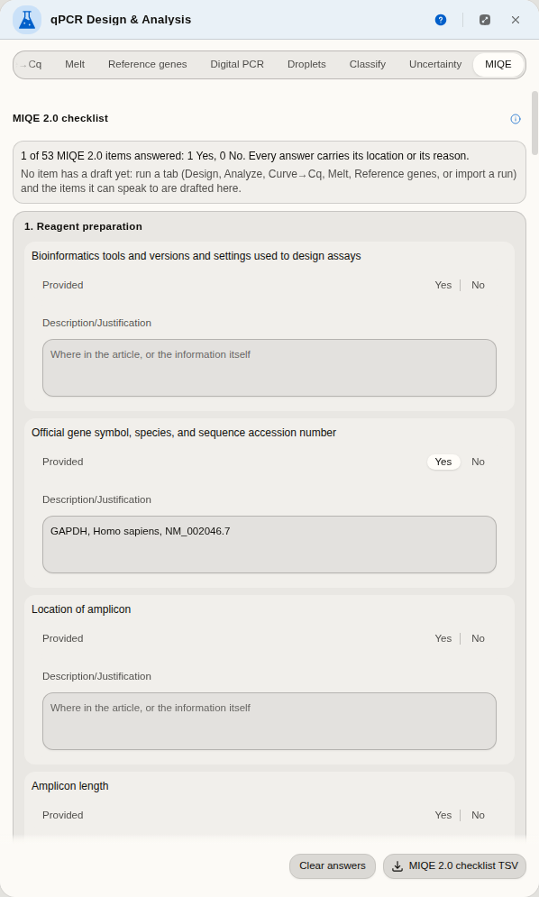
the MIQE 2.0 checklist (Bustin et al. 2025), every item of its Table 1 in the paper's own words and sections, with its two columns: Provided (Yes or No) and Description or justification. Items your runs here can speak to (amplicon location, length and oligo sequences, the raw-data deposit, the Cq method, the efficiency of each standard curve, the quantification model, reference-gene validation, normalisation, the significance test, specificity) open with a drafted description that says which tab it came from. The checklist counts what is answered and names every answer that still lacks a location (Yes) or a reason (No), which is what the table's own footnote asks for
When you'd use this
Used in: Design primers, simulate the PCR, and predict the band
You are measuring how much of a transcript is present, and you want a number you can defend. Typically: design the assay against your target's sequence → run the plate → import the instrument file → fit the curves to get Cq → normalise against a reference gene → and finally state the result with an interval rather than as a bare fold change.
For absolute quantification without a standard curve, the Digital PCR tab takes partition counts instead. For confirming a single product, the Melt tab reads the dissociation curves.
Where it lives
Tools → qPCR Design & Analysis opens the panel beside the sequence view. The Design tab reads whatever you have selected on the sequence — select a region and it designs against that region, or switch the target to the whole sequence. Primers and probes it designs can be written back onto the map as annotations, so the assay is visible on the molecule rather than only in a table.
Before you commit to one, turn on Show on map under the assay you have selected. The amplicon, both primers and the probe are drawn on the molecule straight away, and nothing is saved — the marks are a preview, so you can step down a list of ranked assays and watch each one land on the gene before deciding. Where the amplicon sits matters as much as its numbers do: an assay that looks best on Tm and dimer scores can still straddle the wrong exon boundary, sit on a known variant, or fall outside the region your primers have to reach. Add primers + probe to map is the separate, deliberate action that writes real annotations you keep.
Digital PCR opens the same panel on its own tab.
Inputs and outputs
In. An instrument export in RDML (every published version, v1.0 through v1.4, as an .rdml/.rdm archive or a bare XML file) or an Applied Biosystems .eds experiment archive from QuantStudio, or plain tables you can paste from a spreadsheet — Cq values, amplification curves, melt curves, partition counts, or a table of replicate measurements. Design needs a nucleotide sequence open.
Out. Every result table exports as CSV, and the MIQE 2.0 checklist as TSV. Designed assays can be added to the sequence as annotations, and amplification, melt and standard curves are drawn so you can check a fit by eye rather than trusting a number. And the run itself goes back out as RDML — your melting temperatures, exclusion verdicts and notes written into the fields the format defines for them, so the next person to open the file in their own software sees the analysis rather than the raw curves.
What it refuses, and says so. A tab tells you what is missing before you press its button, next to the control that chose it — a target region shorter than the minimum amplicon, a well table with no partition counts, a melt file that states no expected melting temperature, an expression whose variables you have not given values for. An empty results table is never the way you find out something was wrong.
Step by step
One experiment, end to end, with the result handed between tabs rather than retyped. Open the qPCR & digital PCR sample project — it opens on human GAPDH, the reference gene every other number in this project is normalised against, with the panel already beside it.
1. Read the instrument file in
Import → Load example run. A real RDML v1.4 export: one run, 47 reactions, amplification curves, melt curves and the instrument's own Cq values. The summary tells you what the file holds before you commit to anything, and each destination is its own button.
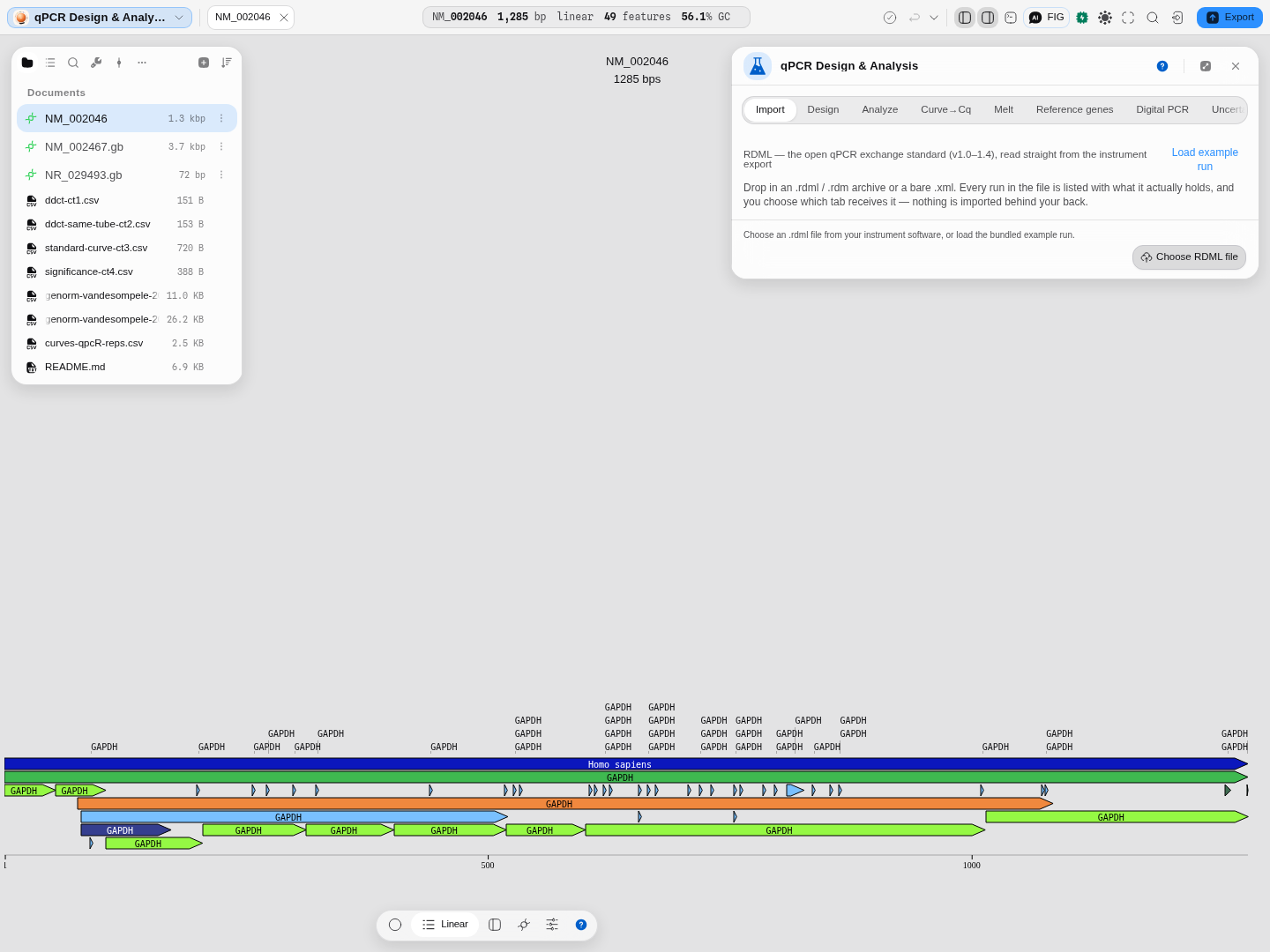
A destination that cannot work is disabled with the reason underneath — this file has no partition counts, so Digital PCR is greyed out instead of failing later.
2. Turn curves into Cq — and check the fits
Send 47 curves → Curve→Cq, tick Choose the model automatically, press Fit → Cq. Read the
marks before the numbers: ✕ is a fit that describes no amplification (14 of 47 here — the
inhibited dilutions), ⚠ is a well unlike its group.
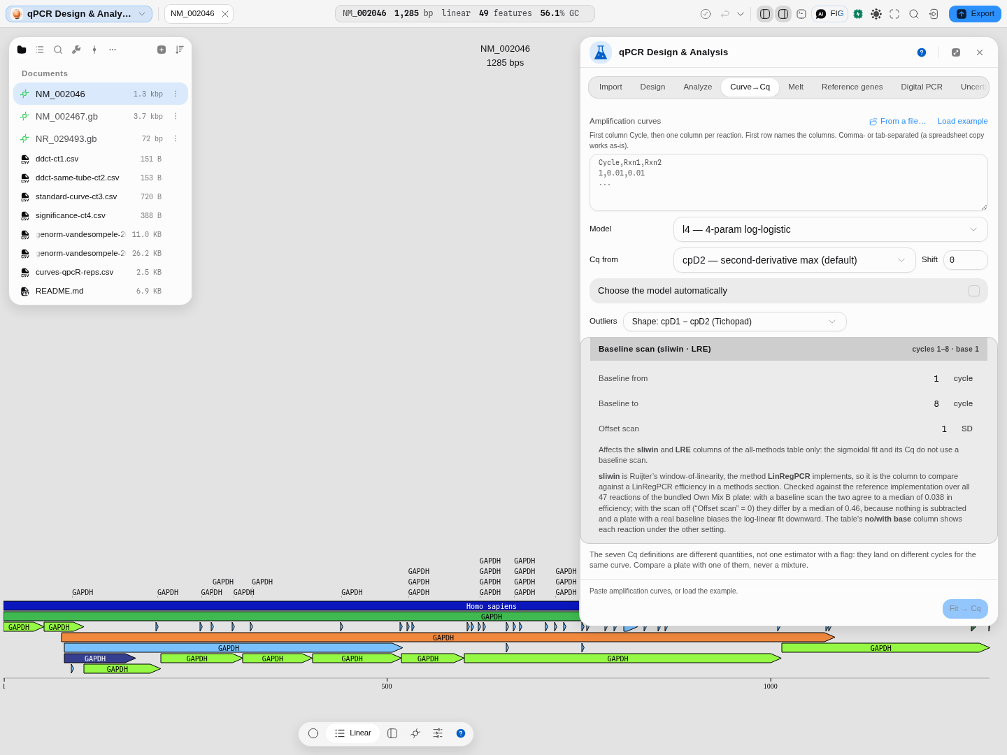
Reaction C11: Cq 25.27, efficiency 57.7 %, R² 1.0000. The full treatment of this tab is in Amplification Curves → Cq.
3. Confirm you amplified one product
Melt → Load example run → Analyse melt curves. Forty of fifty wells return a product peak within a degree of the target's declared 85.34 °C; the other ten are named individually with what is wrong.
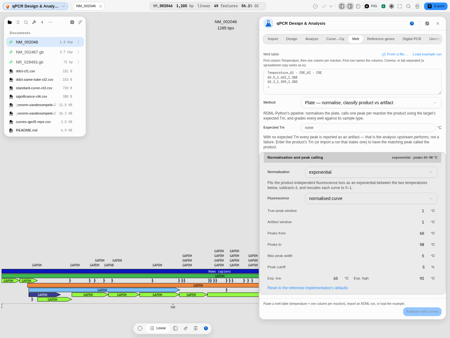
A Cq tells you how much of something amplified. This is the step that tells you what. Details: Melt Curves → Tm.
4. Check your reference genes before you normalise against them
Reference genes → Load example → Rank reference genes. This is the step most protocols skip by picking GAPDH out of habit, and it is the one where being wrong quietly rescales every fold change you report.
Four different algorithms rank your candidates, all in one run, because they routinely disagree and no single one of them is the field's answer:
- geNorm (Vandesompele 2002) — the M statistic, computed by repeatedly eliminating the least stable gene. It also answers a question the others do not: how many reference genes you need, from the pairwise-variation V.
- NormFinder (Andersen 2004) — a variance-components model. Give it a Group column (tissue, treatment, timepoint) and it separates variation within your groups from systematic drift between them, which is the failure geNorm and BestKeeper cannot see: a gene that is beautifully steady inside each group and shifted between them will normalise your comparison away.
- BestKeeper (Pfaffl 2004) — descriptive statistics of the raw Cq plus each gene's correlation with the BestKeeper index. Ranks on the mean absolute deviation of Cq.
- Comparative ΔCt (Silver 2006) — the mean, over every other gene, of the spread of the paired ΔCt.
The headline is the RefFinder consensus (Xie 2012): the geometric mean of each gene's rank across the four. Lowest wins.
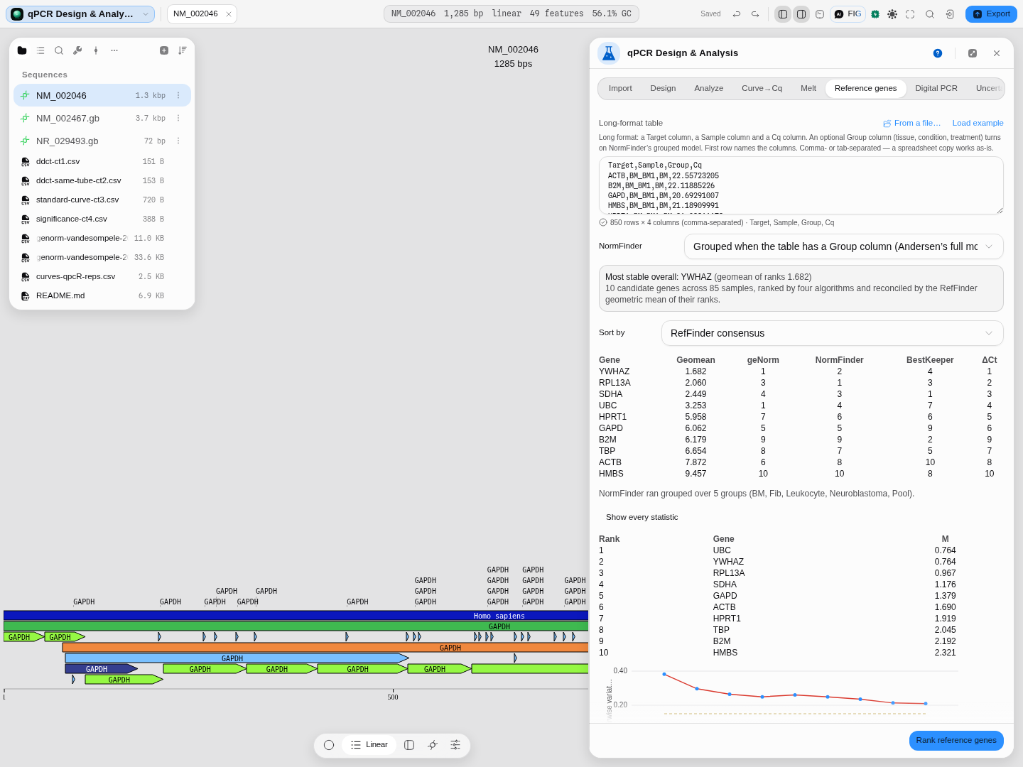
YWHAZ is most stable overall at a rank geomean of 1.682 — but read the columns, not just the answer. BestKeeper puts SDHA first and YWHAZ fourth; geNorm cannot separate YWHAZ from UBC at all. That disagreement is information, and it is why all four are shown.
Pro tip: add a Group column. Without it NormFinder falls back to a variance-only estimate, which is a different and weaker question. With it, the Show every statistic section gives you a per-group bias table — how far each gene drifts in each tissue — which is usually the most actionable thing on the panel.
A pitfall the panel will tell you about: on some datasets NormFinder's ungrouped arm and the comparative ΔCt method return the identical ranking, in which case the consensus is really counting one opinion twice out of four. When that happens it says so on the run.
Does the ranking hold in every condition? With a Group column the tab also runs geNorm inside each group and asks whether those rankings agree, using Kendall's W (0 when the conditions order the genes independently, 1 when they all give the same order), Friedman's χ² and a permutation p that shuffles each condition's ranks. On the five Vandesompele 2002 tissues W is 0.44 against 0.20 by chance (permutation p about 0.01): the conditions agree more than chance, far from perfectly. GAPD has the best mean rank (2.7, never below 5), while RPL13A goes from the top two in bone marrow to ninth in neuroblastoma. A gene with a good mean rank and a bad worst rank is stable on average and unsafe in the condition where it ranks worst. geNorm cannot order its final two genes, so they share rank 1.5 in every condition, and the χ² tie correction counts that.
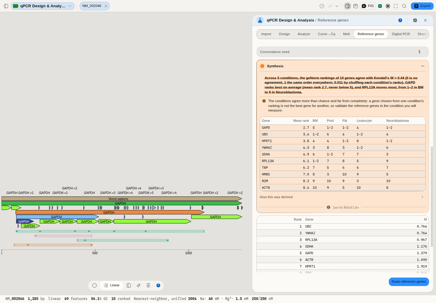
Once you have an answer, Use <gene> in Analyze carries it straight to the quantification tab as the reference gene, so the decision and the normalisation cannot drift apart.
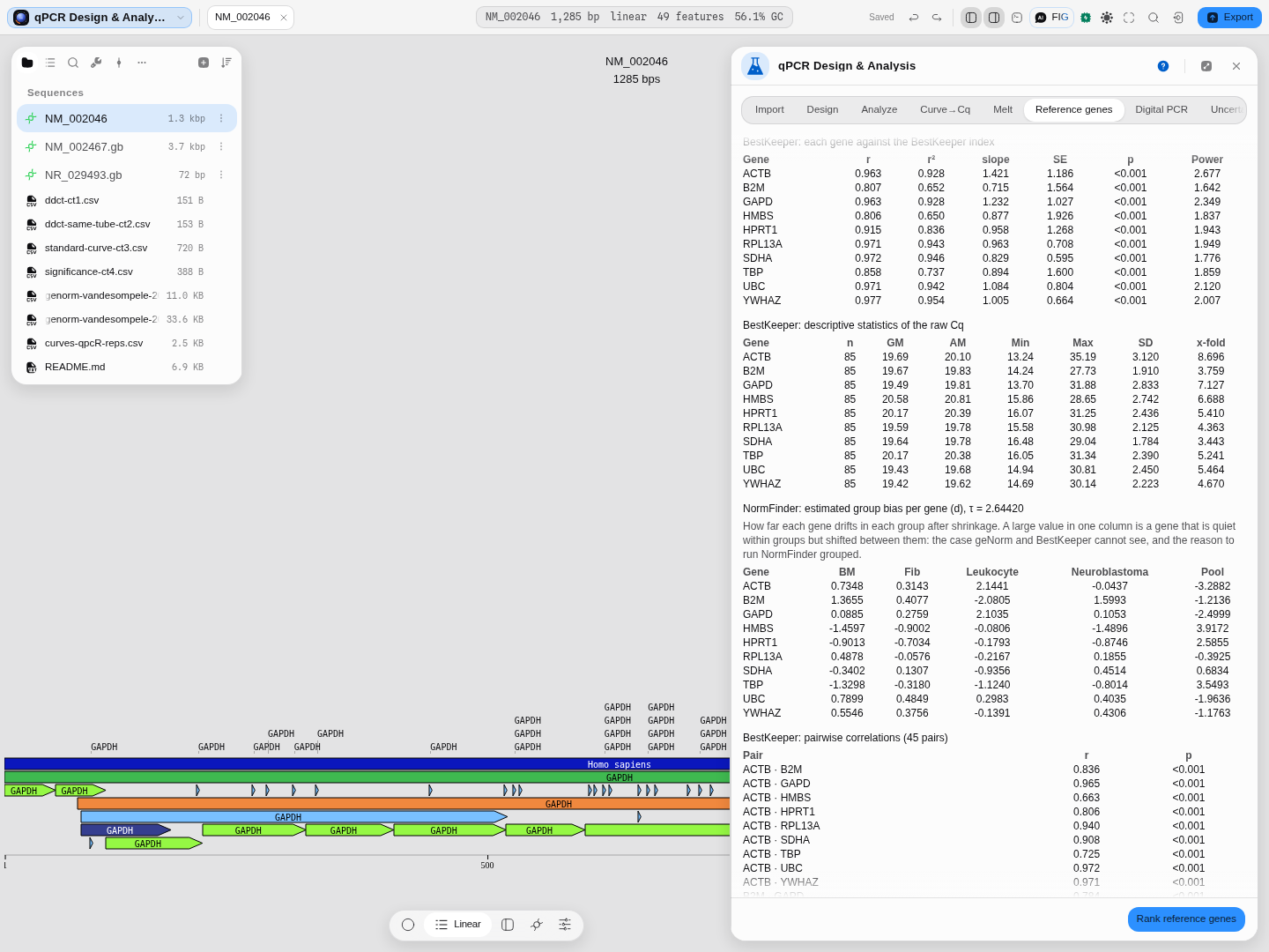
Nothing is hidden behind the ranking: every number each of the four algorithms computed is one click away.
5. Quantify
Analyze → ΔΔCt → Analyze. A real published dataset: c-myc against GAPDH in brain and kidney, six replicates each, separate tubes. Kidney comes back at 5.64 relative to brain.
Set Significance to a test if you want one — Welch t-test, linear model, or the full Wilcoxon rank-sum surface with its exact null distribution and Hodges-Lehmann estimate.
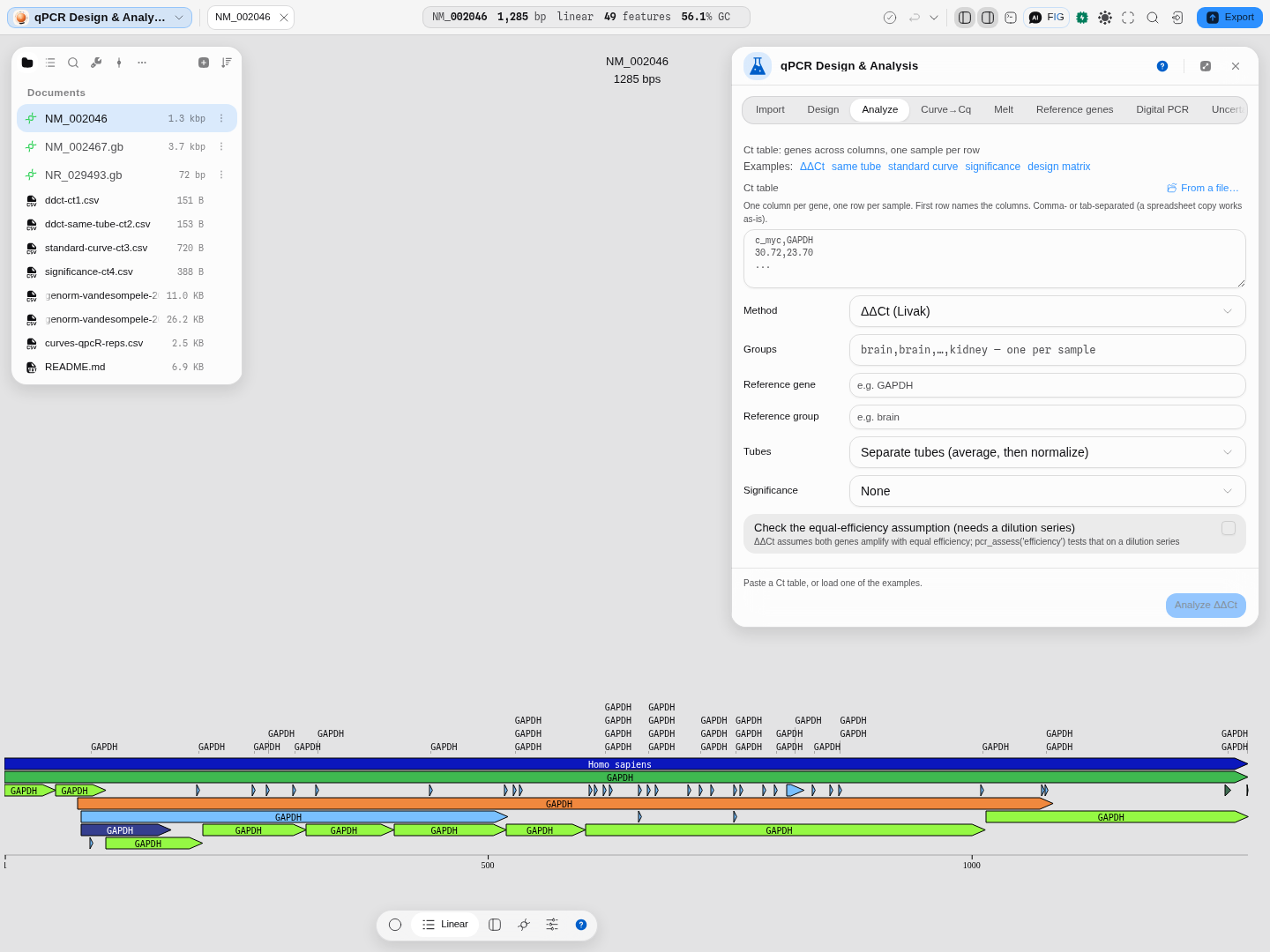
The significance block appears with every knob the test has, not a single p-value.
6. Say how precise that number is
Uncertainty → Seed from Analyze. It carries the two quantities and their standard deviations across; the expression is their ratio. Press Propagate uncertainty.
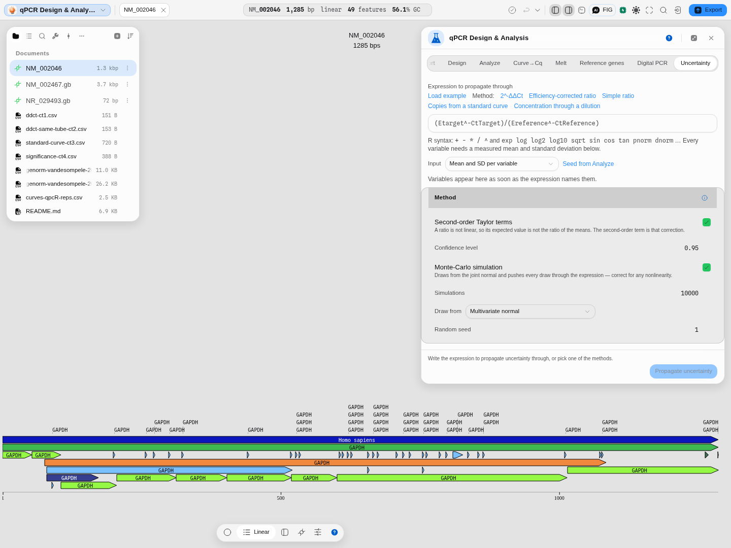
Propagated and Monte-Carlo agree (0.1167–0.2382 against 0.1162–0.2388), which is how you know the ratio is close enough to linear over this spread for the analytic answer to be trustworthy.
And read the share column. 99.1 % of the uncertainty comes from the brain measurement — so repeating the kidney one would buy you almost nothing. That is the sentence that decides what you do at the bench next.
7. Or skip the ratio entirely
If your question is absolute rather than relative, Digital PCR takes partition counts instead of Cq values and gives copies per microlitre with no standard curve — see Digital PCR.
8. Fill in the MIQE 2.0 checklist
MIQE lists every item a journal asks a qPCR author to report, from the MIQE 2.0 revision's own Table 1, in its five sections. Each item has the paper's Provided choice and a Description or justification field. Where an earlier step produced the answer (the standard curves' slopes and efficiencies, the reference-gene ranking, the Cq method, the instrument file), the description is drafted from that run and says so. A draft is not an answer: Provided stays empty until you choose Yes or No, because only you know where in the article the information is. MIQE 2.0 does not rank its items as essential or desirable, so none is marked as optional here. Export TSV saves the checklist under the paper's column headers, ready for a submission. A digital PCR experiment reports against dMIQE 2020 instead.
Worked example
Open the qPCR & digital PCR sample project. On the Analyze tab press ΔΔCt to load a real published dataset: c-myc measured against GAPDH in brain and kidney, six replicates each, run in separate tubes. Press Analyze. Kidney comes back at 5.64 ± 0.10 relative to brain.
Now switch to Uncertainty and press Seed from Analyze. It fills in the two quantities and their standard deviations. The expression is the ratio of them. Press Propagate uncertainty:
- brain / kidney = 0.1774, standard deviation 0.0310
- analytic 95 % interval 0.1167 – 0.2382
- simulated 95 % interval 0.1162 – 0.2388
- 99.1 % of the uncertainty comes from the brain measurement
The same run on screen: the two quantities and their standard deviations carried over from Analyze, and the three-arm summary underneath.
The two intervals agreeing tells you the ratio is close enough to linear over this spread that the analytic answer is trustworthy. The 99.1 % tells you which measurement to repeat if you want a tighter number — repeating the kidney one would buy you almost nothing.
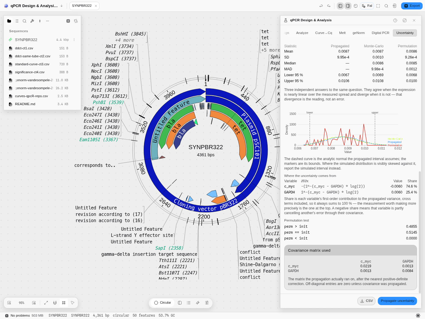
Press Load example instead and you get the replicate path: six real replicate measurements of two genes, with the covariance between them propagated and the permutation arm active. Its density is spiky because six rows can only resample into finitely many values — smoothing that would be drawing a distribution the data does not have.
Will these oligos work together?
A qPCR assay fails most often for a reason no Tm or GC number predicts: the oligos anneal to each other. A forward and reverse primer that pair at their 3′ ends extend into a primer-dimer, which amplifies beautifully, melts at its own temperature and shows up in SYBR as signal you will read as template. A probe that dimerises with a primer is consumed and simply costs you signal.
Every designed assay is therefore checked for structure, and the result travels with it:
- Hairpin — the oligo folding on itself. Above 24 °C it competes with template annealing.
- Self and Self 3′ — the oligo pairing with a copy of itself, anywhere and at its 3′ end. The 3′ one matters more: that is the configuration a polymerase can extend.
- For+Rev, For+Pro, Rev+Pro — the three cross-pairs.
For+Revat the 3′ end is the classic primer-dimer.
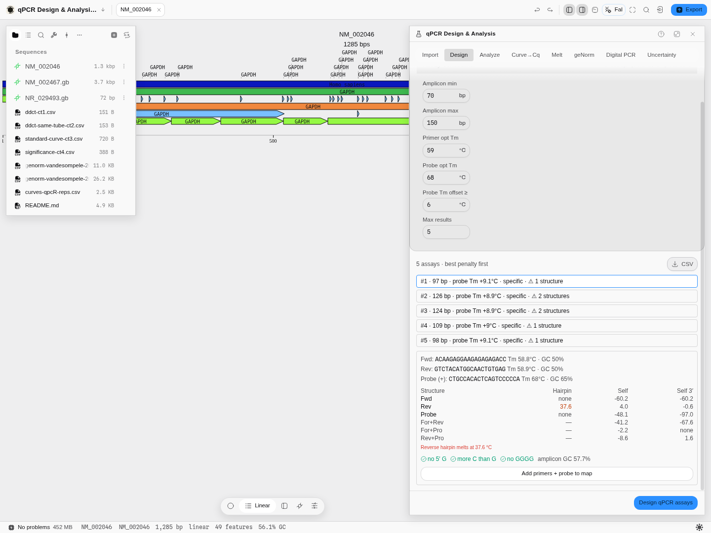
Numbers are melting temperatures in °C. none means no structure was found at all — the good case, and one a temperature cannot express. A structure that melts well below your annealing temperature has already come apart before the primer is asked to work, which is why large negative numbers are harmless. Here the reverse primer's hairpin melts at 37.6 °C, above the 24 °C limit, and is called out in words underneath; the assay list marks how many structures each assay has, so you can choose a clean one before you open it.
The thresholds are primer3's own — 24 °C for a hairpin, 45 °C for a self-dimer anywhere, 35 °C at a 3′ end — not values chosen here, and the same engine and limits the primer designer and the multiplex pooler use, so a ΔG quoted in one panel agrees with the others. The structures melt under your reaction conditions, not a default: change the salt and the temperatures move.
Can these assays share a tube?
With more than one assay designed, Check which assays can share a tube scores every pair. Two questions are being asked at once, and they have different answers:
- Do the primers of the two assays anneal to each other? That makes primer-dimer in a tube containing both.
- Does a primer of one assay anneal inside the other's amplicon? For assays designed against the same gene this is the likelier problem, because their amplicons overlap — and it is the one a primer-dimer check alone cannot see.
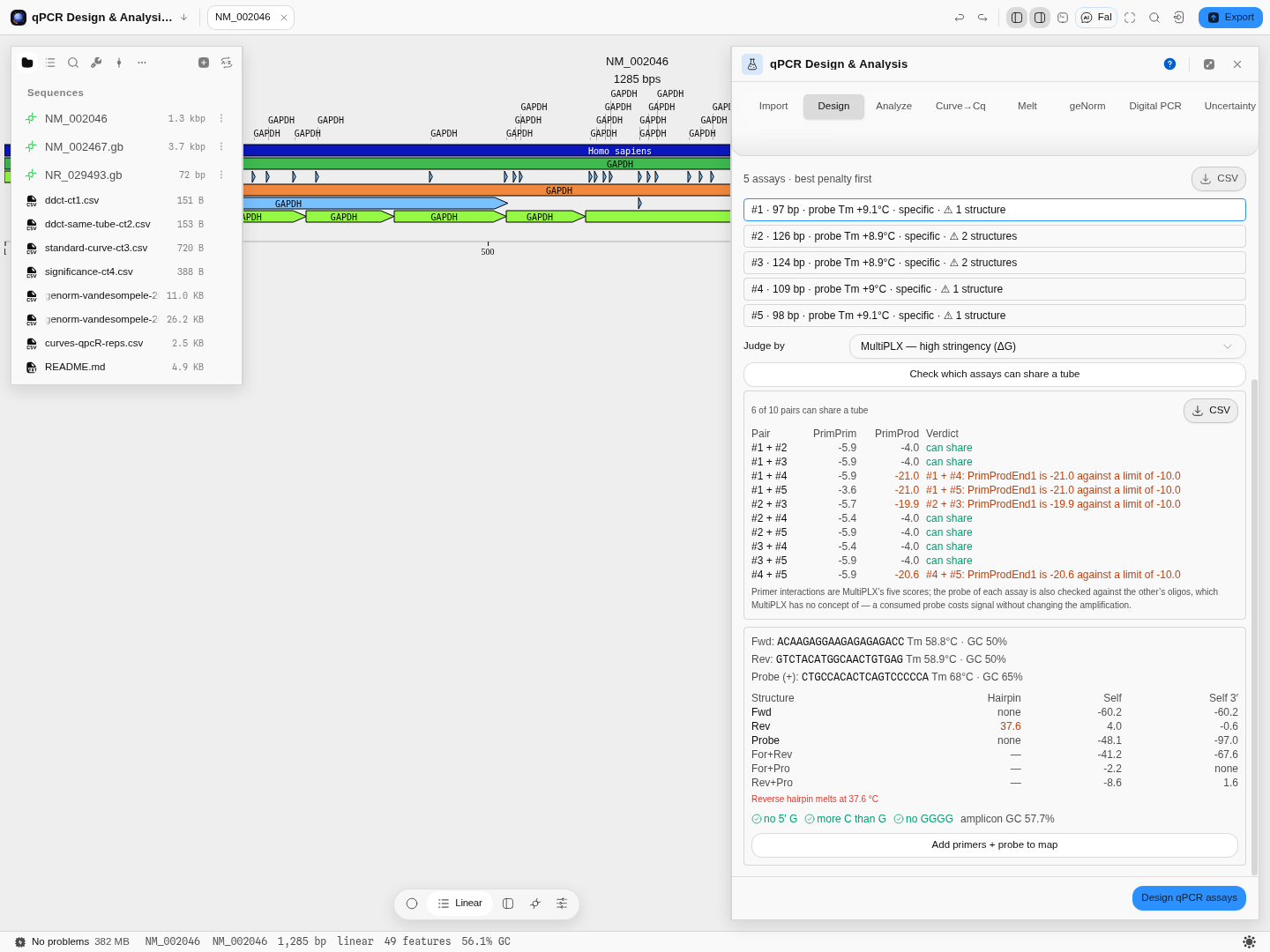
Five assays on one transcript, judged by MultiPLX's high-stringency cutoffs: six of the ten pairs can share a tube, and each of the other four is named by the limit it breaks — a primer sitting inside its partner's product at −21.0 kcal/mol against a −10.0 cutoff. Judged instead by primer3's dimer limits, all ten pairs pass, because primer3 defines no primer-product limit.
Which is right? Both, for different questions — which is why Judge by is a control rather than a hidden default. primer3's limits are melting temperatures calibrated for the engine that computes these numbers. MultiPLX's are free energies from a tool built specifically for multiplex pools, and they cover the primer-product interactions primer3 does not. If you are pooling assays from one gene, use a MultiPLX stringency; the primer3 verdict will look reassuring and is answering a narrower question.
Each assay's probe is also checked against the other assay's oligos — something neither tool models, because neither has a probe. A probe consumed by a neighbour's primer costs signal without changing amplification, so it looks like poor efficiency and gets blamed on the primers.
How to act on a warning. A flagged hairpin or self-dimer usually means picking a different assay from the list — that is what the list's structure count is for. A 3′ cross-dimer between the two primers is the one never to ignore: it is a product that will amplify.
Controls
Design — amplicon length range, primer and probe melting-temperature windows, GC content, poly-X runs, and TaqMan probe chemistry. Every constraint is a field, not a hidden default.
Import — every run in the file is listed with what it holds (how many amplification curves, melt curves, instrument Cq values, partition counts), and each destination is offered only if the run actually has the data for it.
Curve → Cq — eight sigmoid models (or automatic model choice), all seven Cq definitions, the exponential-phase window, and four independent efficiency estimators reported side by side.
Analyze — ΔΔCt, ΔCt or standard-curve quantification; same-tube or separate-tube; the reference gene and reference group; an optional equal-efficiency check; and a choice of significance test.
Melt — the normalisation method, the peak window and width, the temperature cutoff, and the expected melting temperature to classify against. All five stages of the analysis are drawable and downloadable.
Digital PCR — partition volume, reaction and template volumes, the dilution chain, whether replicate wells are pooled, and which confidence-interval method to use.
Uncertainty — the expression, the confidence level, first- or second-order expansion, Monte-Carlo on or off with the number of draws and the choice of a plain or truncated normal, permutation on or off with the number of permutations and which columns are tied together, whether to propagate the measured covariance, and the random seed so a simulated run can be reproduced exactly.
Every control, by tab
The tables use the panel's own labels. A default of empty means the field starts blank and the run waits for you to fill it.
Design
| Control | Default | What it sets |
|---|---|---|
| Target sequence | empty | A sequence to design against instead of the editor selection |
| Max results | 5 | How many ranked assays are returned |
| Probe chemistry | DNA | DNA or LNA. The probe's backbone, which changes its melting temperature |
| Locked bases | empty | With LNA, which probe positions are locked, counted from 1 at the 5′ end |
| Check secondary structure (hairpins and cross-dimers) | on | Rejects assays whose oligos fold or pair with each other |
| Fwd · Rev | from the chosen assay | The primer pair, with the probe, that the readouts below describe |
Import
| Control | What it sets |
|---|---|
| Run | Which experiment and run in an RDML file to open, each listed with its reaction count |
| Reporter dye | For a QuantStudio .eds file, the dye whose signal is read |
| Passive reference | None: use the raw reporter signal, or divide by a passive dye to get Rn |
Curve → Cq
| Control | Default | What it sets |
|---|---|---|
| Amplification curves | empty | A pasted table of cycle-by-cycle fluorescence, one column per reaction |
| Criterion | Nested F-test (within family) | How the automatic model choice compares fits. Also Likelihood ratio (within family), AICc weights (all eight models), Reduced chi-square (needs replicates) |
| E(x) | off | Overlays the per-cycle efficiency curve on a reaction's plot |
| Baseline from · Baseline to | cycles 1–8 | The cycles the baseline is fitted over for the window-of-linearity and LRE estimators |
| Offset scan | 1 SD | How far the baseline search scans, in standard deviations of the background |
| Contributing reactions | Grubbs | Which reactions set a target's mean efficiency: Grubbs (LinRegPCR's own choice, drops outliers), Median window, or All |
| Window half-width | 0.05 | With Median window, how far from the median efficiency a reaction may sit and still count |
| Iterations | 200 | Bootstrap resamples behind a Cq's error bar |
| Observations dropped | 1 | How many cycles the jackknife leaves out at a time |
| Resample the readouts | on | Resamples the Cq definitions, efficiency and initial fluorescence too. Off resamples the model coefficients alone, which is faster |
Reference genes
| Control | Default | What it sets |
|---|---|---|
| Long-format table | empty | A Target column, a Sample column and a Cq column. An optional Group column turns on NormFinder's grouped model |
| Sort by | — | Orders the candidate genes by one method's ranking: RefFinder consensus, geNorm (M), NormFinder, BestKeeper (SD of Cq) or Comparative ΔCt |
| Concordance permutations | 999 | Shuffles of each condition's ranks when the table has a Group column |
| Concordance seed | 1 | Fixes the shuffles so a run reproduces exactly |
Analyze
| Control | Default | What it sets |
|---|---|---|
| Ct table | empty | The Cq values to quantify |
| Groups | empty | Which sample belongs to which group |
| Reference gene | empty | The gene every target is normalized to |
| Reference group | empty | The group every other is compared with |
| Tubes | Separate tubes (average, then normalize) | Or Same tube (normalize per reaction), when target and reference were amplified in one reaction |
| Alternative | Two-sided | The Wilcoxon test's alternative: Two-sided, Less (shift < 0), Greater (shift > 0) |
| Null dist. | Auto (exact if both groups < 50) | Or Exact conditional, or Normal approximation |
| Tail corr. | Continuity | None, Continuity, or Continuity plus an Edgeworth term of order 1, 2 or 3 |
| Coverage | 0.95 | The confidence level of the reported interval |
| Formula | ~ group | The linear model, in R formula notation, over the variables below |
| Variables | empty | A table of the covariates the formula names |
| Normalize | Subtract (ΔCt = target − reference) | Or Divide (target ÷ reference) |
| Check the equal-efficiency assumption (needs a dilution series) | off | ΔΔCt assumes both genes amplify with equal efficiency; this tests it |
| Serial-dilution Ct table | empty | The dilution series the efficiency check and the standard curve read |
| Input amounts | empty | The amount of template in each dilution |
Melt
| Control | Default | What it sets |
|---|---|---|
| Melt table | empty | Pasted temperature and fluorescence readings |
| Expected Tm | none | The melting temperature this assay should produce, which each peak is classified against |
| View | Normalized | Raw fluorescence, Smoothed, Normalized, −dF/dT (first derivative) or Second derivative |
| Well | the first | Which well the plots show |
| Target | Every target | On the plate heatmap, which target's reading each well shows |
| True-peak window · Artifact window | 1 °C · 1 °C | How wide a peak is integrated when it is the product, and when it is an artifact |
| Peaks from · Peaks to | 60 · 98 °C | The range peaks are called in |
| Max peak width | 5 °C | Broader peaks are not called |
| Peak cutoff | 5 % | Peaks smaller than this share of the tallest are dropped |
| Exp. low · Exp. high | 65 · 92 °C | The range the exponential background model is fitted over |
| Bilin. low from · Bilin. low to | 65 · 67 °C | The low baseline of the two-line (bilinear) normalization |
| Bilin. high from · Bilin. high to | 93 · 94 °C | Its high baseline |
| Coefficient of variation as a percentage | on | Off reports replicate spread as a fraction |
| Smoother span | 0.05 | Fraction of points in the super smoother's window on the derivative curve |
| Peak window | 51 points | The odd window of the running-maximum peak detector. Even values are rounded up |
| Min peak area | 0 | Peaks with less area are dropped |
| Window ceiling | 8 points | The largest neighborhood the derivative search may pick, between 2 and 8. Every width up to it is fitted and the best adjusted R² wins |
| Report the two inflection points | off | The negative and positive peaks of the second derivative. Their distance is the transition width, which separates one clean transition from two overlapping ones |
| List every peak, not just the largest | off | Every local maximum and minimum of the smoothed derivative, so a secondary product shows as a second maximum |
| Show peaks above | 10 % of the tallest | A display floor on that list |
| Pre-smooth the raw curve | off | A smoothing spline before differentiation. Off by default because smoothing moves the Tm |
| Degrees of freedom | 0.95 × GCV | The spline's stiffness, as a fraction of what generalized cross-validation chose |
| Subtract a linear background | off | Fits a straight line over the range below and subtracts it |
| Background from · to | this run's coolest fifth | The temperature range of that line |
| Rescale onto 0–1 | off | Min-max normalization after the background step, so curves of different amplitude share an axis. It does not move the Tm |
Digital PCR
| Control | Default | What it sets |
|---|---|---|
| Partition table | empty | One row per well: well, sample, target, then the positive and accepted partition counts |
| Dilution factor | 1 | Multiplies the concentration back to the undiluted sample |
| Volume CV | 0 % | Spread of partition volumes, which widens the interval |
| Merge replicate wells of the same sample + target (pools counts, not λ) | on | Pools the partition counts of replicate wells before estimating |
| Reference copies | 2 copies/genome | Copies of the reference per genome, for copy-number calls |
Droplets
| Control | Default | What it sets |
|---|---|---|
| Droplet amplitudes | empty | Two-channel amplitudes, one droplet per row |
| X channel name · Y channel name | HEX · FAM | Which columns are which dye |
| Lowest empty fraction · Highest empty fraction | 0.3 · 0.99 | A well is rejected when its empty population is too small to be the empty droplets, or so large that no positive population is left to quantify |
| Droplets to classify | empty | One well's two amplitude columns, Ch1 then Ch2, to sort into the four two-target populations |
| Neighbors (k) | 5 | How many nearest droplets of the labeled training well vote on each one |
Uncertainty
| Control | Default | What it sets |
|---|---|---|
| Expression | empty | The quantity to propagate, written over named variables |
| Input | Mean and SD per variable | Or Replicate observations, pasted under Replicate measurements |
| Replicate measurements | empty | One column per variable |
| Propagate the measured covariance | off | Replicates measured in one tube co-vary; ignoring that misstates the spread |
| Second-order Taylor terms | on | A ratio is not linear, so its expected value is not the ratio of the means |
| Monte-Carlo simulation | on | Pushes random draws through the expression, correct for any nonlinearity |
| Simulations | 10,000 | How many draws |
| Draw from | Multivariate normal | Or Truncated at the 95 % bounds |
| Permutations | 2,000 | Draws of the permutation test |
| Tie groups (one number per column, same size per group) | empty | Which columns are permuted together |
Algorithms you can choose
Cq definition — seven of them, and they are genuinely different quantities, not one method with a flag: the second-derivative maximum, the first-derivative maximum, the point of maximum efficiency, an efficiency-threshold crossing, Cy0, CQ, and maxRatio. The second-derivative maximum is the default because it needs no threshold you have to pick.
Quantification — ΔΔCt (Livak & Schmittgen 2001) assumes both assays amplify at 100 % efficiency. The efficiency-corrected ratio (Pfaffl 2001) uses each assay's own measured efficiency instead. The standard-curve method quantifies against a dilution series you ran yourself, and matches curves to samples by gene name so a target is never quantified against another gene's curve.
Reference-gene stability — four algorithms and their consensus, run together: geNorm's M statistic and pairwise variation V (with the 0.15 cutoff drawn), NormFinder in both its ungrouped and grouped forms, BestKeeper, the comparative ΔCt method, and the RefFinder geometric mean of all four rankings. Every statistic each of them computes is available, not just the rank.
Amplification efficiency — four independent estimators reported side by side for every reaction, because agreement between them is the evidence a well is clean: from the fitted sigmoid, the window-of-linearity on log₁₀(fluorescence), an exponential-phase fit, and the linear regression of efficiency (LRE). The window-of-linearity column is the method LinRegPCR implements, so it is the one to compare against a LinRegPCR efficiency in someone's methods section. Whether a baseline is subtracted moves that estimator by far more than the difference between any two of the four, so the panel shows each reaction under both settings.
Kinetic outlier detection — five tests, and they ask different questions. Two are univariate: the shape test (cpD1 − cpD2, Tichopad 2010) and an efficiency Z-score against the group (Bar 2003). Three are multivariate, scoring each curve against a robust covariance of the whole plate: cpD1 against the cpD2 residual (Tichopad MOD1), slope and Fmax (Tichopad MOD2), and slope, fluorescence at cpD1 and Fmax (Sisti 2010). The third sees something the second cannot — a reaction that rose at a normal rate to a normal plateau but crossed at the wrong fluorescence.
Melt — two engines answering two questions. One is an instrument-grade plate analysis that classifies every well against the target's expected melting temperature; the other reports every melting peak with the area under it and calls the largest as the dominant product.
Confidence intervals for digital PCR — ten methods, from the exact Clopper–Pearson interval through Wilson, logit, probit, complementary log-log and the others, to a Bayesian highest-density interval on a Jeffreys prior and a likelihood-ratio interval. They converge at moderate occupancy and separate at the extremes, which is exactly where a digital run needs the choice to be yours.
Uncertainty — three independent answers to the same question, computed together so you can see whether they agree:
- the analytic expansion, exact for a linear expression and corrected to second order for one that is not;
- Monte-Carlo, which draws from the joint distribution of your inputs and pushes every draw through the expression, so it is correct for any nonlinearity;
- permutation, which resamples your actual replicates and assumes no distribution at all.
The science
Cq from a curve. An amplification curve is fitted with a sigmoid, and the Cq is read off the fitted model rather than off a threshold line you place by eye. Different Cq definitions read different features of the same fitted curve, which is why they give different numbers on the same well and why the choice is exposed.
Reference-gene stability, and why four algorithms. Each of the four measures a different kind of steadiness. geNorm asks which genes co-vary most tightly with each other; NormFinder asks which has the least variance once you separate within-group from between-group; BestKeeper asks which varies least in absolute Cq and tracks the plate's overall signal; comparative ΔCt asks which has the smallest average pairwise spread. On real data they disagree, and picking whichever one supports your habitual housekeeping gene is exactly the failure the consensus exists to prevent. Worth knowing: comparative ΔCt is mathematically geNorm's M before any elimination, so on a plate whose ranking is stable under elimination those two are not independent opinions.
Amplification efficiency and the baseline. The window-of-linearity method fits a straight line to the log of fluorescence over the exponential phase. That log is only meaningful once the background fluorescence has been subtracted — with no baseline subtraction on a plate whose background sits in the tens of thousands of fluorescence units, the fitted slope is biased downward and the efficiency comes out substantially too low. The baseline scan is therefore on by default and exposed as a control, and each reaction is shown under both settings so you can see how much of your efficiency is the curve and how much is the baseline.
Robust outlier detection. The multivariate tests measure each curve's distance from the centre of the plate — but the centre and spread are estimated with a minimum-covariance-determinant estimator, which is computed from the most concentrated half of the reactions. That matters because a classical mean and covariance are dragged towards the very outliers you are trying to find, so a plate with two bad wells can end up flagging neither. The cut-off then adapts to the plate: it moves outward only when the tail of the distance distribution genuinely exceeds what chance would produce.
Relative quantification. ΔΔCt is a ratio of two exponentials, so its uncertainty does not behave like a difference of Cq values. Both the equal-efficiency form and the efficiency-corrected form are offered because the first is only valid when the assumption behind it holds — and the panel can test that assumption on a dilution series rather than leaving you to assume it.
Absolute quantification. In digital PCR the reaction is split into partitions and the positives are counted. Because a positive partition may have held more than one molecule, the concentration is recovered from the negative fraction: λ = −ln(1 − k/n) copies per partition, then divided by the partition volume. dMIQE 2020 asks for the partition volume to be reported, so it is a field rather than a constant, and occupancy outside roughly 10–95 % is flagged because precision falls away at both ends.
Melting analysis. The dissociation curve is smoothed, normalised and differentiated; peaks in the negative first derivative are melting transitions. A single sharp peak near the expected temperature is one product; extra peaks are primer-dimer or non-specific amplification. The measured temperature is shown next to the temperature predicted from the amplicon's own sequence, so a disagreement is visible rather than inferred.
Error propagation. Any quantity you compute from measured numbers inherits their uncertainty, and how it inherits it depends on the shape of the expression. To first order, the variance of f(x₁…xₙ) is GΣGᵀ — the gradient of f at your measured means, times the covariance of your measurements. When f is curved, that underestimates it, so a second-order term built from the exact Hessian is added. A ratio is curved, which is why its expected value is not quite the ratio of the means and why the second-order correction is on by default.
The panel also decomposes that variance across your inputs, so each measurement's share of the total is reported. Cross terms are included, so the shares always sum to 100 %; a negative share means that measurement is partly cancelling another's error through their covariance, which happens when two things were measured in the same tube.
Where your inputs are correlated — and replicates measured together usually are — that covariance is propagated rather than assumed away. It is measured from your replicates, and adjusted to the nearest valid covariance matrix if the measurement produces one that is not (a covariance estimated from incomplete pairs need not be).
Provenance. The curve fitting, Cq definitions, relative quantification, significance tests, reference-gene stability, melting analysis, digital-PCR quantification, the confidence-interval methods and the error propagation are all checked against the published R implementations of those methods — value for value, including the derivatives, the covariance handling and the random draws — and against the RDML consortium's own reference reader for instrument files — in both directions. The .eds reader is checked the same way, against the only open reader of that format, value for value over every well of every real instrument export that reader ships with. A
file this tool writes is read back by that reference implementation and compared value for value with
the original, and validated against the consortium's published schema for its version, across every
file of their own published corpus plus real exports from an ABI StepOne, a Roche LightCycler 96 and
a Bio-Rad CFX.
Limitations
Specificity does not extend past the open sequence. Primer and probe candidates are filtered on melting temperature, GC content and repeats and on TaqMan chemistry rules, and every oligo and cross-pair is then scored thermodynamically for hairpins and dimers — see above. What the search cannot tell you is whether a primer binds somewhere else in a genome it has never been shown.
Specificity is checked against the sequence you have open, not against a genome. The panel says so where it reports it. A genome-wide specificity check is a different capability.
Minor-groove-binder (MGB) probes have no melting-temperature model here, and that is a statement about the literature rather than about this tool. Locked nucleic acid and Scorpion chemistries are both supported, because both have a published parameter set to stand on. MGB does not: the canonical measurements report anything from +10 °C to +49 °C depending on how A/T-rich the site is, because the ligand binds the A+T-rich minor groove, so no single offset can be right and a guessed one would silently shift every design.
Digital PCR starts from counts. Re-thresholding raw droplet amplitudes ("rain" analysis) is not done. Partition volume is taken as constant at the value you enter, which is what every platform reports; a per-platform volume-variance correction needs values no vendor publishes.
Melting analysis compares against an expected temperature only when your file states one. When it does not, every peak is honestly reported as unclassified rather than being assigned a product identity.
The forward simulation is singleplex, and its defaults are one assay's. It models one target per run — the published model says in as many words that multiplex competition would need substantial additions — so it cannot tell you what two assays do to each other in one tube. Its primer-dimer free energy is a quantity computed with NUPACK, which this tool does not carry: the value it starts from belongs to the model's own reference assay and you should replace it with one computed for yours. Its association rate constants were fitted on that reference assay, not measured, and the result says so beside every number.
Uncertainty. Propagation assumes your inputs are normally distributed around their measured means — the truncated-normal option limits the tails, but it does not change that assumption. The permutation arm makes no distributional assumption but needs real replicates, so it is offered only when you supply them. Expressions may use arithmetic, powers, exponentials, logarithms, roots, trigonometric functions and the normal density and distribution functions; gamma-family functions are refused with a message rather than approximated.
Compared with other tools
We ship more of the method than the instrument software does, and we say which parts are checked against what.
More curve models, and a test that picks between them. Eight sigmoidal models are fitted here — four-, five-, six- and seven-parameter logistic and the same four Baranyi shapes — and the panel will run a nested F-test, an Akaike-weight comparison, a residual-variance ratio or a χ² test to tell you which one your curve actually justifies. Instrument packages typically fit one shape and never mention it.
Seven Cq definitions, side by side. The second-derivative maximum is the default because it is the one most instruments approximate, but cpD1, maxE, expR, Cy0, CQ and maxRatio are all computed from the same fit and shown together, so a Cq that moves by a cycle when you change definition is visible rather than hidden inside a vendor's algorithm.
An interval on the Cq itself. A fitted Cq is an estimate, and almost nothing reports its uncertainty. Here you can resample the curve — residual bootstrap or jackknife — and get a confidence interval on cpD1, cpD2 and the per-reaction efficiency, plus a converged-fraction readout so a curve that only fits half the time says so instead of returning a confident number.
Ten binomial confidence intervals on a digital PCR count, including Bayesian HDI and a likelihood-ratio interval, rather than the single Wilson or exact interval a platform hard-codes. At the extremes — a handful of positives, or a nearly saturated plate — the choice moves the reported concentration, so it is a control on the panel and not a hidden default.
Two melt engines, because they answer different questions. Plate-level analysis with product and artifact verdicts, and a per-curve Tm with peak area off a spline derivative. Most software offers the first only.
Uncertainty on anything you compute downstream. Type in the expression you actually publish — a ratio, a dilution chain, a normalised concentration — and get first- and second-order propagation, a Monte-Carlo simulation and a permutation test on the same inputs, with the variance contribution of each term. That is a step most workflows do in a spreadsheet, without an error term.
Checked against the reference implementations, byte for byte. Curve fitting, efficiency, model selection, outlier detection, melt analysis, propagation and the resampling intervals are all validated against the published R packages that define them, and the digital PCR intervals against the R implementations of each interval, with the vectors kept so anyone can re-run the comparison.
What we do not do: we do not drive an instrument, and we do not re-threshold raw droplet amplitudes.
We now read one run file that has no published schema. An Applied Biosystems .eds is opened
directly — both the generations QuantStudio software has written — and what comes out is the
instrument's own dye-decomposed fluorescence, well by well and cycle by cycle, with the plate
geometry read from the file rather than guessed from how many wells happen to hold data. Two things
about it are worth knowing before you rely on it. You choose the reporter dye and the passive
reference, because a normalised reading is the reporter divided by the reference and the file
names its dyes without saying which one is passive; on these instruments it is conventionally ROX,
and some runs have none. And a file saved before its analysis is refused by name rather than
opened as an empty plate — a run still in progress looks exactly like a finished one until you look
for the analysed fluorescence, which is not there.
For anything else, bring an RDML export or a table.
Export
Every result table leaves as CSV, and the run itself leaves as RDML.
Writing results back into the file. A qPCR analysis usually ends as a spreadsheet sitting next to the instrument file, which is where it stops being findable. RDML has fields for what a melt curve tells you, so Import → Write results back and export puts them there:
| Field | What goes in it |
|---|---|
meltTemp | The melting temperature of the product peak. The format holds one temperature per reaction, so any artifact peaks go into the note rather than being dropped. |
excl | Why a reaction was excluded — the same field the instrument and LinRegPCR read when they leave a well out. |
note | The advisory verdicts, plus every artifact peak's temperature. |
corrF | The product peak's share of the reaction's total signal. LinRegPCR uses this to correct quantities, so it is off by default: switch it on only if that is what you want. |
Each is a switch, and a switch is disabled with the reason when the file's own version has no field
for it — RDML 1.0, 1.1 and 1.2 have no meltTemp or note at all, and writing one would produce a
file that fails its own schema. The report says how many fields were written, and how many cleared
a melting temperature rather than setting one, which is what happens when a file states no expected
Tm for its targets and the analysis therefore calls no peak the product.
Then download it two ways: the .rdml archive, which is what instrument software expects, or the
bare rdml_data.xml, the uncompressed form every RDML reader must also accept. Both carry every
run in the file, not only the one you were looking at.
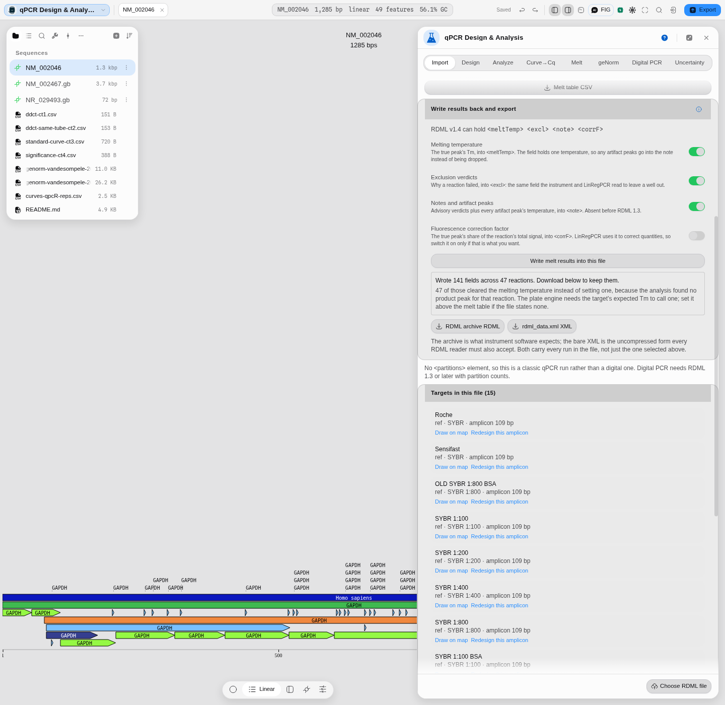
Pitfall worth knowing. If the melt tab is holding a pasted table, or a different file's run, the button says so instead of writing nothing: the reactions have to belong to the run that is loaded.
API
The engine is one interface over six halves, each answering a different question and each checked against the authority named beside it, and each callable on its own with plain JSON in and out:
| Call | What it answers | Checked against |
|---|---|---|
designQpcrAssay | primer pair + hydrolysis probe, ranked by penalty | our own @tm + @primer |
pcrDdct · pcrDct · pcrCurve · pcrStandard · pcrEfficiency | relative quantification from Ct values | R's pcr |
standardCurveFits · efficiencyPercent | the standard curve, and efficiency from its slope | R's pcr |
effCurve · cy0 · efficiency | fitting an amplification curve → Cq and per-reaction efficiency | qpcR |
genorm… | reference-gene stability and normalization factors | geNorm |
meltAnalysis · meltQpcR · meltMBmca | three melt engines, three questions (see below) | RDML-Python · qpcR · MBmca |
dpcr… · binomProfile | digital PCR absolute quantification | dpcR / binom / rateratio.test |
import { pcrDdct, standardCurveFits, efficiencyPercent } from '@ports/qpcr';

const rows = pcrDdct(ctInput, { group, reference, referenceGroup });
const fits = standardCurveFits(ctInput, amounts);
const eff  = efficiencyPercent(fits[0].slope);   // 100% at slope −3.32
Three melt engines is the point, not redundancy. meltAnalysis is instrument-grade plate
analysis with product/artifact verdicts; meltQpcR gives per-curve Tm and peak area off a
spline derivative (R's own Fortran supsmu, ported); meltMBmca gives a sub-grid Tm as the
vertex of the best-fitting quadratic near the extremum, with the fit quality that produced it.
Asking "what is the Tm" of one curve and "did this plate work" are different questions, and the
package keeps them apart rather than averaging them into one number.
Everything is JSON-serializable on purpose: this crosses the bundle boundary and may run in a worker, so the engine stays pure and the app owns the state.
Automation
- Workflow DAG: the design half is
design_qpcr_assay, categorydesign, a write node. Parameters:max_results(best penalty first) and every one of the twenty design constraints, with the amplicon window and the two target melting temperatures to hand and the rest — the length, temperature and GC windows for primer and probe, and the single-base run limit — under Advanced. The secondary-structure check is a parameter too. The panel and the graph read the same list, so a constraint you can set in one you can set in the other. - A seventh node,
check_scorpion_stem, takes a probe element, its loop's target and a stem length, and returns both melting temperatures, their difference, the stem's GC and a verdict against whatever margin you pass — with the margin's provenance returned beside it, so a rule of thumb cannot be read downstream as a measured specification. - Outputs:
assays(ranked),count,best, and the three sequences of the best assay —forward,reverse,probe— so an oligo order wires straight into the next node. - The analysis half is five more nodes, added 2026-09-03 so a plate can be taken apart in a
pipeline and not only in the tab:
call_cq(amplification curves to a Cq per reaction, under any of the eight sigmoids and any of the seven Cq definitions, with the fit-quality block beside the number),relative_expression(all three relative-quantification models, both tube designs, with the fold-change bounds and, on request, a significance test beside them),rank_reference_genes(all four stability algorithms and their consensus, plus the pairwise variation that answers how many reference genes this experiment needs),quantify_dpcr(partition counts to copies per microlitre, eleven interval methods, the occupancy QC beside every reading) andanalyze_melt_curves(peaks and a per-reaction verdict against an expected melting temperature, or an explicit refusal to classify without one). - Each takes the table the tab takes, read by the same reader, and opens on the same defaults the tab opens on — so a plate pasted into the panel and the same plate wired into a graph are quantified against the same droplet volume, the same baseline window and the same model.
- Every control the tab has, the node has (widened 2026-09-03 from a quarter of them). Curve→Cq
carries automatic model selection and its ranking criterion, the kinetic-outlier test, and the
baseline-scan window with its offset. Melt analysis carries all three of its engines and each
engine's own knobs. Digital PCR carries the target-vs-reference copy number and the reference
ploidy. Reference genes carries the NormFinder arm —
autoor forced ungrouped, which are two different questions rather than a fallback, and the result says which one ran. - Relative quantification is the whole tab, not the easy model. You can ask for the standard-curve method, which fits each gene's own serial dilution and converts every Ct to an input amount before taking a ratio — the model to use when the two assays do not amplify at the same efficiency, and the one a delta-delta-Ct pipeline silently cannot express. You can run a significance test in the same call: Welch's t-test, the equivalent linear model, the Wilcoxon rank-sum test with its alternative, exactness rule, tail correction and coverage all yours to set, or a design-matrix linear model for an experiment the two-group comparison cannot describe — a dose series, a batch term, an interaction — written as a formula against a table of your own variables. And you can ask for the equal-efficiency check on the same run, which regresses delta-Ct on log₁₀ template per gene and tells you whether delta-delta-Ct was the right model at all rather than leaving you to assume it was.
- They return what the tab shows, not a headline number: the model ranking, the four-estimator comparison with each failure named, the outlier verdicts including the reactions the test could not measure, the reactions whose baseline crosses zero, the copy-number interval rescaled onto the concentration scale it belongs to, and the replicate spread of the readings.
- The copilot calls them all by the same names with the same parameters and the same approval gate.
- Nothing on the analysis side is panel-only any more. This section used to say the Uncertainty tab and the Cq error bars were, on the reasoning that both need a fitted curve handed between steps. That was wrong about both. Error propagation never sees a fitted curve at all — it takes an expression and a table of numbers, which is what every other step here takes — and the resampling builds its fit from the same pasted amplification table the panel does, so the fit was never something a pipeline had to supply. Both are now steps you can wire, on the same parameters the panel offers. The uncertainty step also reports which measurement to make more precisely: it returns each variable's share of the total variance, which is the question the panel's derivative table answers and the one a pipeline usually wants back.
- Batch is
pcrBatch/batchToRows, which run one analysis across many targets and flatten the result to rows for a CSV.
Provenance
What a run records is the question: which files were imported and how their columns were mapped, which Cq definition was used, which wells were excluded and why, the reference gene(s) and reference group, the efficiency assumed or measured, and the model behind every fit. Those are what another lab needs; the numbers are a pure function of them.
Exclusions are part of the record, not a private edit. A dropped well stays visible as dropped with its reason, because a quantification computed over a silently trimmed plate is the one result nobody can reproduce.
The three melt engines are named in the output, so a Tm carries which of them produced it — plate analysis, spline-derivative peak, or the sub-grid quadratic vertex with its fit quality. Two Tms from two engines are not a disagreement to average; they answer different questions, and the provenance says which was asked.
A predicted curve says which of its inputs were measured and which were fitted. The forward simulation implements the kinetic model of Kreitmann et al., Analytical Chemistry 2026, 98(12), 9089-9101, and is checked against that work's own reference implementation on its own assay. Not every number in it is the same kind of quantity, so the result lists them separately: the binding constants are nearest-neighbour thermodynamics evaluated in the stated salt; the primer-dimer free energy is a NUPACK quantity belonging to the reference assay, which you should replace with one for yours; and the association rate constants were fitted by that work's optimiser on its own data, not measured. Quoting a predicted Cq without saying which is how a fitted parameter becomes a constant in somebody's methods section.
Citing the method: name the engine as well as the statistic. Relative quantification is a port
of R's pcr; curve fitting and per-reaction efficiency of qpcR; reference-gene stability of
geNorm; the melt engines of RDML-Python, qpcR and MBmca; digital PCR of dpcR
with binom/rateratio.test; the forward simulation of DYNAMIC. Each is checked against that
library, and the comparison can be re-run, so a reviewer can re-derive the numbers rather than
trust them.
Screenshots
Every tab is shown in context in the walkthrough above, seeded and run, rather than listed here as a gallery of resting states. Two frames that do not appear there:
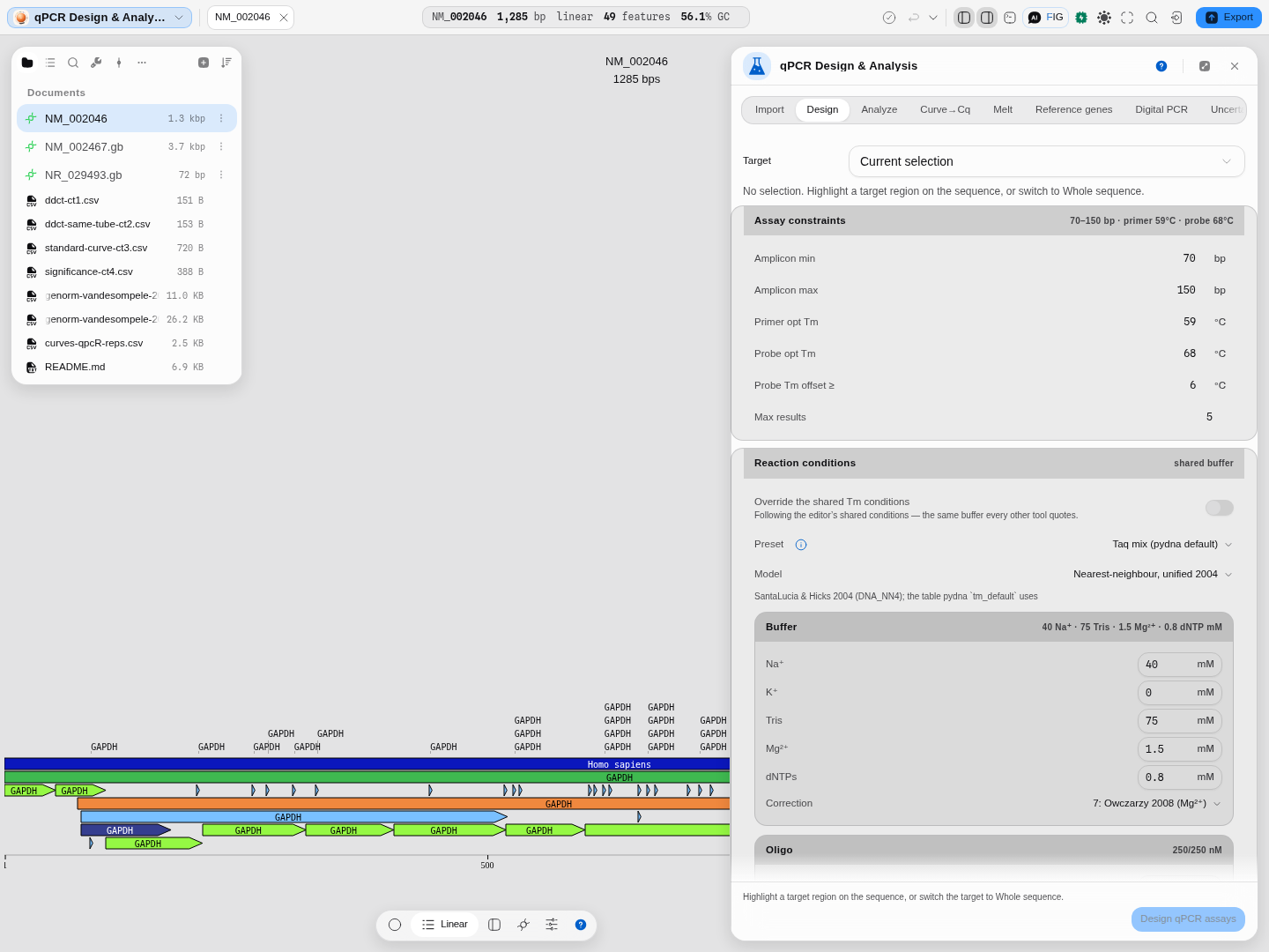
Design is the one tab that reads the sequence on the stage — and writes back to it, so the assay is visible on the molecule rather than only in a table.
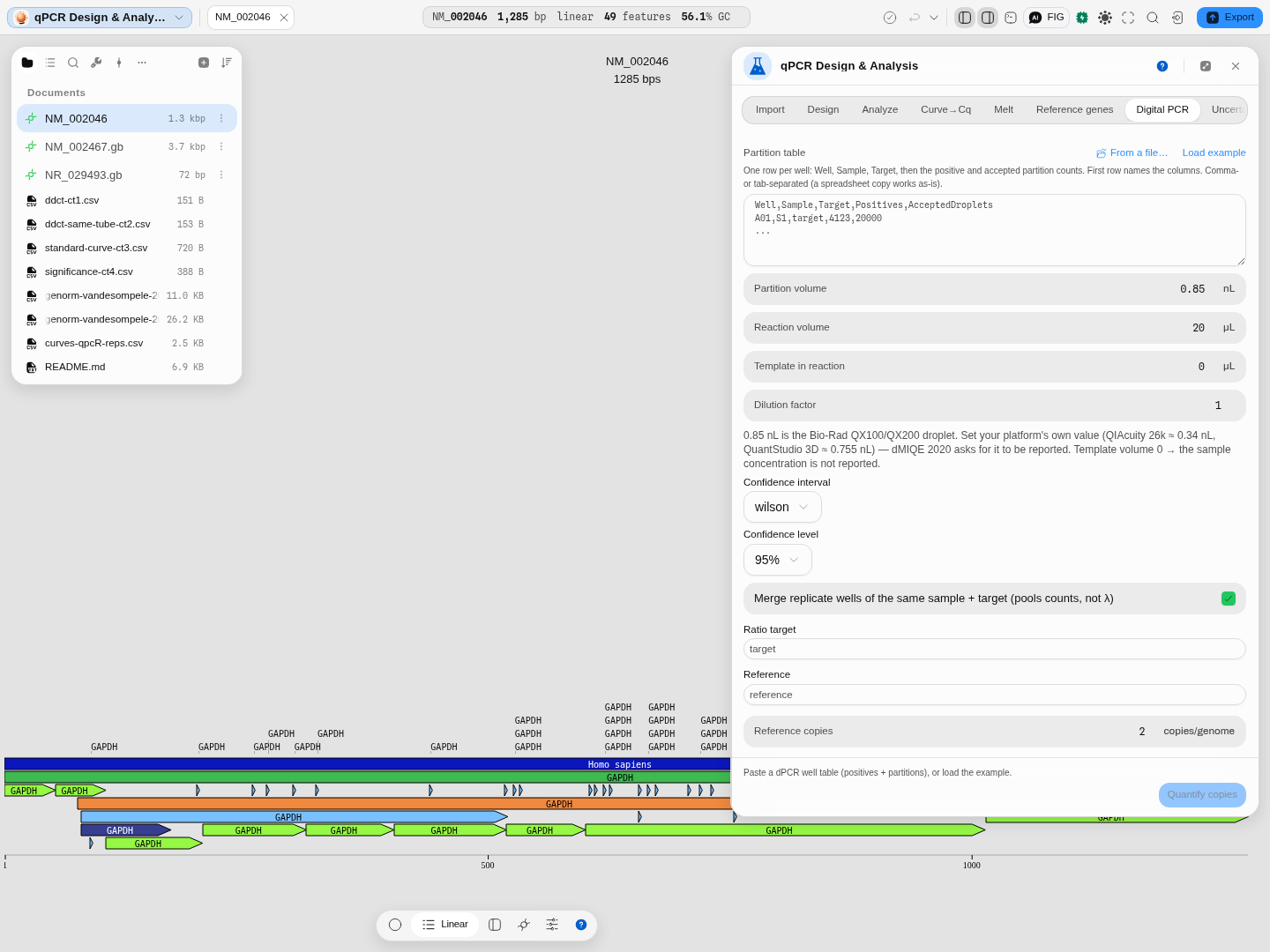
Digital PCR takes counts rather than Cq values, so it is the one tab that does not need anything from the steps above.
Related
In this group: Primer Designer · LAMP primer set · Bisulfite methylation primers · Degenerate primers from an alignment · CODEHOP hybrid primers from a protein alignment · Primer Library · PCR Simulation · Fusion PCR · Multiplex PCR · Digital PCR · Amplification Curves → Cq · Melt Curves → Tm · Droplet gating → concentration · Droplet classification · Melting Temperature