
Melt Curves → Tm
Read the dissociation curves and find out whether you amplified one product or several.
| Reached by | Tools → Melt Curves → Tm |
| Sample project | qPCR & digital PCR |
What it does
A Cq tells you how much of something amplified. It does not tell you what. At the end of a SYBR-based run the instrument slowly heats the plate and watches the fluorescence fall as double-stranded product comes apart; each distinct product melts at its own temperature and shows up as a peak in the negative first derivative. One sharp peak near where you expect it means one product. Two peaks, a shoulder, or a peak in your no-template control means something else amplified too, and every Cq on that plate is now a number about an unknown mixture.
This panel turns those curves into peaks, and then into a verdict per well: a product, or an artifact named by what is wrong with it. It also puts the measured melting temperature next to the temperature predicted from the amplicon's own sequence, so you can see whether the thing that melted is the thing you designed.
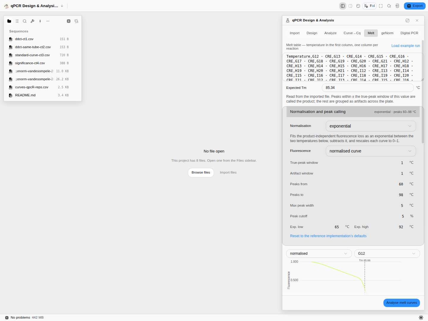
RDML-Python's own 50-reaction CRE plate: 40 of the 50 wells come back with a product peak, mean melting temperature 85.74 °C against the 85.34 °C the file itself states for that target, and the remaining wells are flagged by name rather than quietly averaged in.
What this computes
Per reaction
- a normalised melting curve — the product-independent fluorescence loss fitted and subtracted (exponential, or a bilinear scan that chooses its own windows), then rescaled
- the first and second derivatives of that curve, both downloadable, because the peak everyone quotes is a feature of the first derivative and its edges are features of the second
- every melting peak, with its temperature, width, enthalpy change (ΔH) and the share of the total signal it carries — so a shoulder is a number rather than an impression
- the true peak: the one matched to the target's expected melting temperature, with the window that matched it stated
- verdicts per well — several products, no product at the expected temperature, product in a negative control — each naming its subject
Per target
- the mean melting temperature of the product across the reactions that produced one, the share of wells that did, and the offset from the expected temperature the file states
- the artifact peaks grouped across the plate, so a primer-dimer population is visible as a population
- the melting temperature predicted from the amplicon sequence where the imported file carries it — a Poland–Scheraga calculation in a stated buffer, shown beside the measured value rather than standing in for it
- replicate spread: the location and deviation of each target's replicates temperature by temperature, with the worst coefficient of variation and where it happened — the question a single melting temperature cannot answer
Two engines, two questions. The plate engine normalises and classifies against an expected temperature; the per-curve engine reports every peak with the area under it and calls the largest-area peak the dominant melting temperature. A third method fits a quadratic to the peak vertex for a temperature that does not depend on the sampling grid.
From the vertex method, three further readings — all optional, none of them on by default:
- the two inflection points either side of the melt, read off the second derivative, and the width of the transition between them. A melting temperature says where a transition is; its width says how sharp it is, and a wide one under a single apparent peak is usually two products melting close together rather than one melting badly.
- every local maximum of the smoothed derivative, each with its height as a share of the main peak. A second product appears here as a maximum comparable in height to the first; the many small ones are texture in the derivative, which is why the share is reported and not just a count.
- pre-smoothing, a smoothing spline fitted at a chosen fraction of the degrees of freedom the data itself supports, with an optional linear baseline subtracted over a temperature range you give and an optional rescale onto 0–1. It is off unless you turn it on, because smoothing a curve before differentiating it moves the melting temperature you get out.
Provenance. The vertex method and these three are checked against MBmca — the R package that
defines them, from the surface-melting-curve work of Rödiger, Böhm and Schimke — over every curve in
its own published melt datasets, and the smoothing spline underneath them against R's smooth.spline
on the same curves.
When you'd use this
- Straight after a SYBR run, before you trust a single Cq. This is the check that says whether the run is interpretable at all.
- When a no-template control amplified. The melt curve tells you whether it was primer-dimer (low, broad) or genuine contamination (at your product's temperature) — and those have completely different fixes.
- When you are validating a new assay. The measured temperature against the predicted one is the evidence that the amplicon is the one you designed rather than something else the primers found.
- High-resolution melting work. The peak areas and the full derivative curves are available, not just the peak temperature.
Design the assay in qPCR Design & Analysis; read Cq values in Amplification Curves → Cq.
Where it lives
The Melt tab of the qPCR panel. It reads melt curves, not the sequence on the stage — but it does use the open document in one place worth knowing about: the predicted melting temperature is computed from the amplicon sequence, so what you have open matters for that column.
Inputs and outputs
In: a temperature column and one column per reaction, pasted or imported. Or — much better — a real RDML file from the instrument through the Import tab, which brings the sample types, the target names and the expected melting temperatures with it. Those are what the classifier needs, and a bare table does not carry them.
Out: per reaction, every melting peak with its temperature, height, width and the fluorescence drop across it; which peak was called as the product; the rest grouped into artifact columns that line up across the plate so a shared contaminant is visible as a column rather than as scattered rows; and a verdict per well. Per target, an average. All five stages of the pipeline — raw, smoothed, normalised, first derivative, second derivative — are drawable and downloadable as CSV, so you can check any step rather than trusting the last one.
What it refuses, and says so. Melt analysis needs raw fluorescence. If the file contains baseline-corrected data — which shows up as negative fluorescence — the run is refused with that reason, because normalising an already-corrected curve produces a confident-looking wrong answer. And when a file states no expected melting temperature for a target, every peak is reported honestly as unclassified rather than the largest one being promoted to "the product".
Step by step
1. Load a real melt plate
Open the qPCR & digital PCR sample project, go to Tools → Melt Curves → Tm and press Load example run. It reads a real 50-reaction melt plate. Its CRE target declares an expected melting temperature of 85.34 °C in the file itself — which is what lets the analysis grade each well rather than just measure it.
2. Set the normalisation before you run
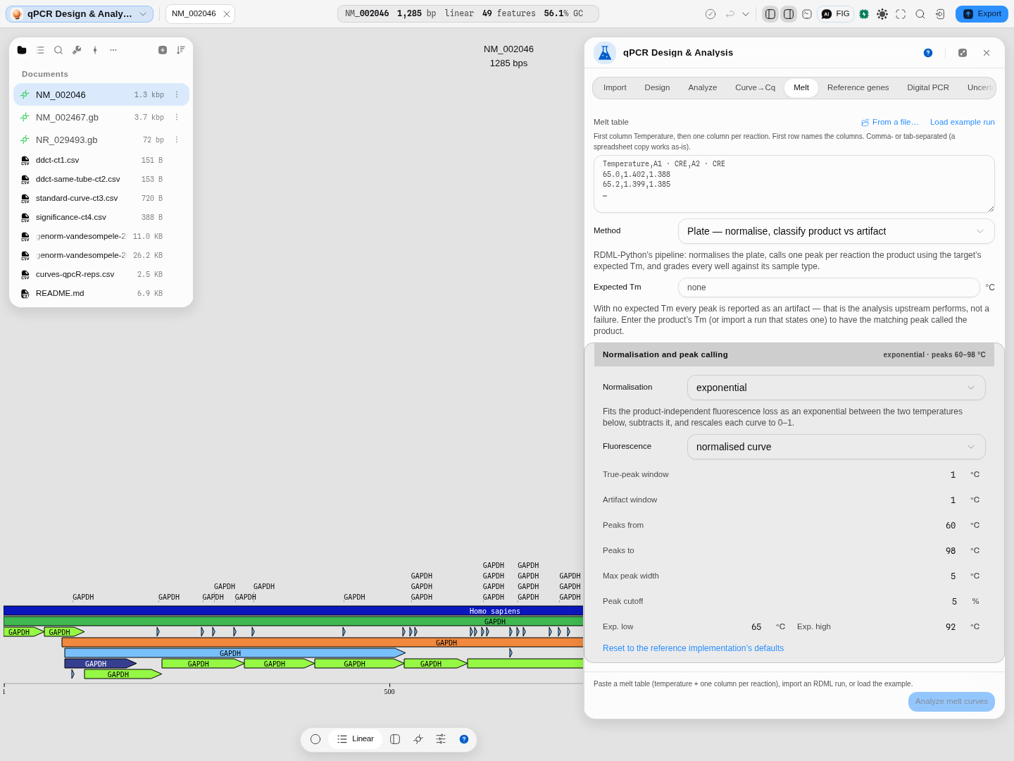
The controls above the button are the analysis, not preferences. Normalization picks how the product-independent fluorescence loss is removed — exponential, bilinear, or both combined — and Fluorescence selects which curve the peaks are called on. The peak-calling window, maximum peak width and area cutoff are all here too, with Reset to the reference implementation's defaults if you want to get back to a known state.
3. Analyse, and read the per-well verdicts
Press Analyse melt curves.
Product in 40 of 50 wells, mean Tm 85.74 °C against the declared 85.34, and two artifact temperatures found across the plate at 74.3 and 79.5 °C.
Forty of the fifty wells come back with a product peak within about a degree of the declared value. The other ten are named, one line each, with what is wrong — "several products with different melting temperatures detected", "no product with expected melting temperature" — rather than silently dropped or returned as a Tm you would have trusted.
4. Cross-check with the second engine
Switch the Method selector to the per-curve engine and run it again. It reports 85.77–85.94 °C where the plate engine called 85.66–85.88 °C.
Two unrelated algorithms, on the same data, landing within two tenths of a degree — which is the real reason to have both. When they disagree, that is information about your curve, not a bug in one of them.
5. Get a sub-grid Tm, with the fit behind it
Switch Method to Vertex — sub-grid Tm + fit quality and press Analyse melt curves again.
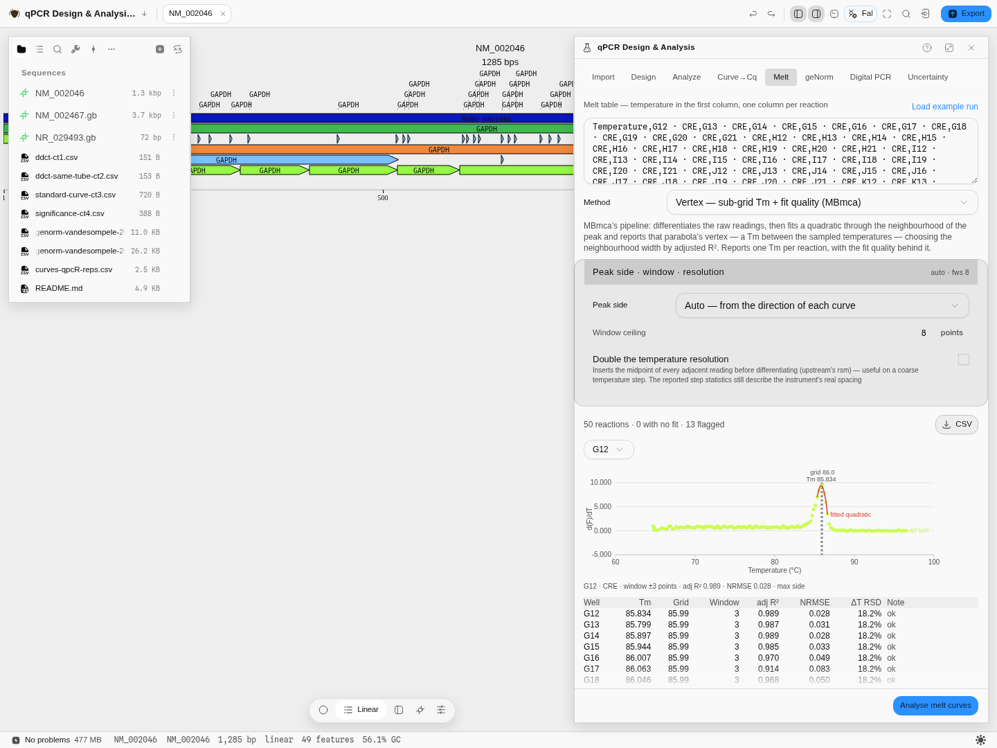
The same 50-reaction CRE plate. Well G12 comes back at 85.834 °C where the raw derivative maximum sits at 85.99 — the gap is the sub-grid correction. The fit that produced it won on adjusted R² 0.989 with a ±3-point window, and its normalised residual error is 0.028. All fifty wells produced a fit; thirteen carry a flag.
Three things on this readout are worth reading every time:
- Tm against Grid. If they are far apart, the peak is not where the quadratic thinks it is — usually a shoulder pulling the fit. The panel flags that case by name.
- adj R² and NRMSE. These grade the fit, not the run. Below 0.85 and above 0.08 respectively are the thresholds the method's own author warns at, and the Note column says so in words.
- ΔT RSD. The relative spread of your temperature step. This plate reads 18.2% — its ramp is not even, which is exactly the condition that makes a sub-grid estimate worth having.
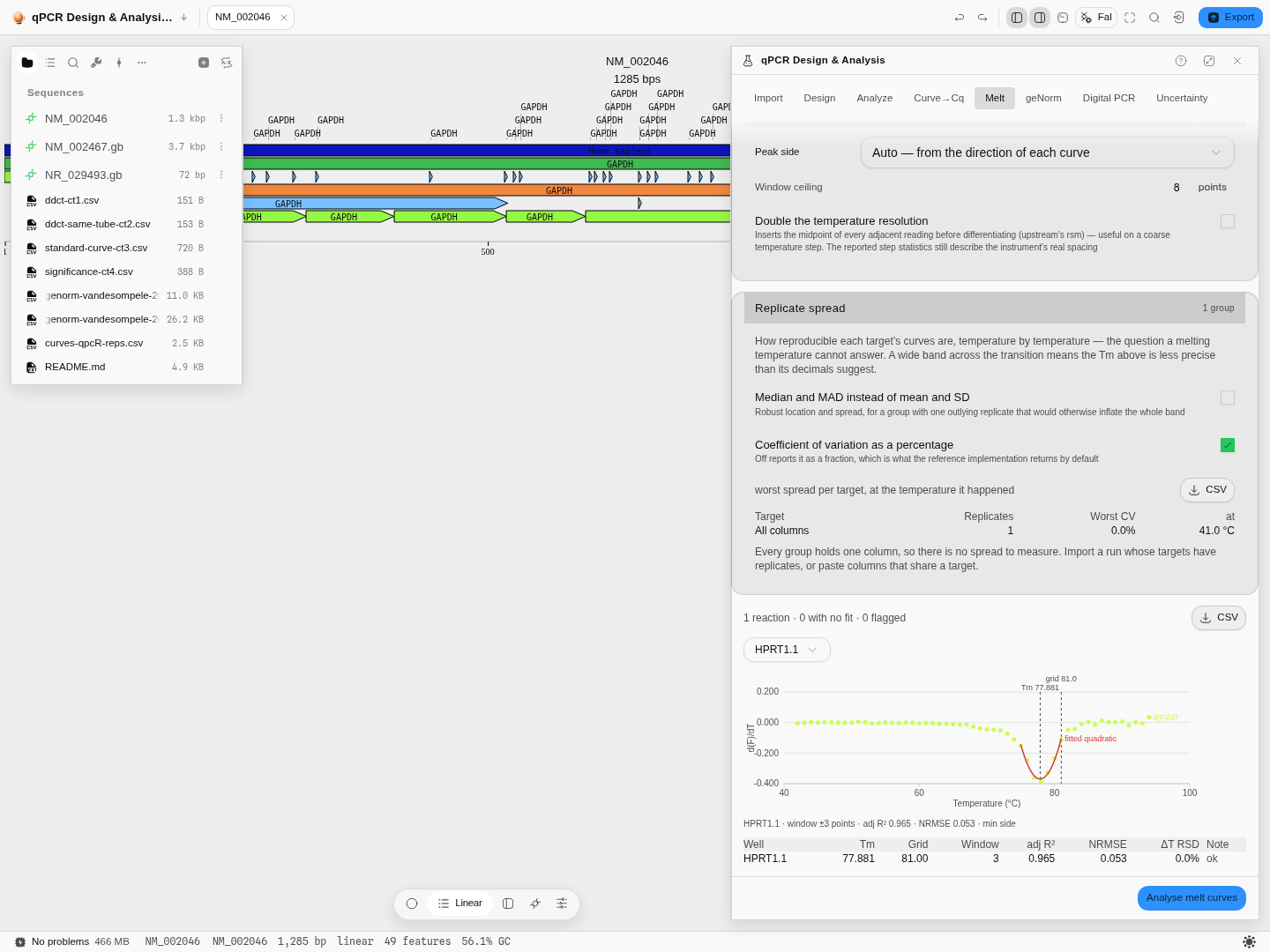
A surface-melting curve whose signal rises instead of falling. Here the melt sits at a minimum of the derivative, and the correction is large: 77.881 °C against a grid maximum of 81.00 — three degrees, because on this curve the sampled points either side of the transition are a full degree apart and none of them sits at the peak. This is the case that makes the method worth choosing.
Peak side is the one control to get right. A melt in solution falls as the dye is released; a
surface or microbead assay rises. The method's own default assumes the rising case, and on a falling
curve it returns a temperature from the far end of the ramp that looks perfectly plausible. Auto
reads the direction of each curve and picks for you, and the line under the plot says which side it
used — on this plate, max side.
Read the ΔT RSD column before you trust three decimals. The rising curve above reports 0.0 % — a perfectly even 1 °C ramp — while the CRE plate reports 18.2 %. An uneven ramp is exactly the condition a sub-grid estimate helps with, and also the condition that makes the raw grid maximum least trustworthy.
Turn on Double the temperature resolution to insert the midpoint of every adjacent reading before differentiating. It is the right move on a coarse ramp and it is not free: it smooths real structure.
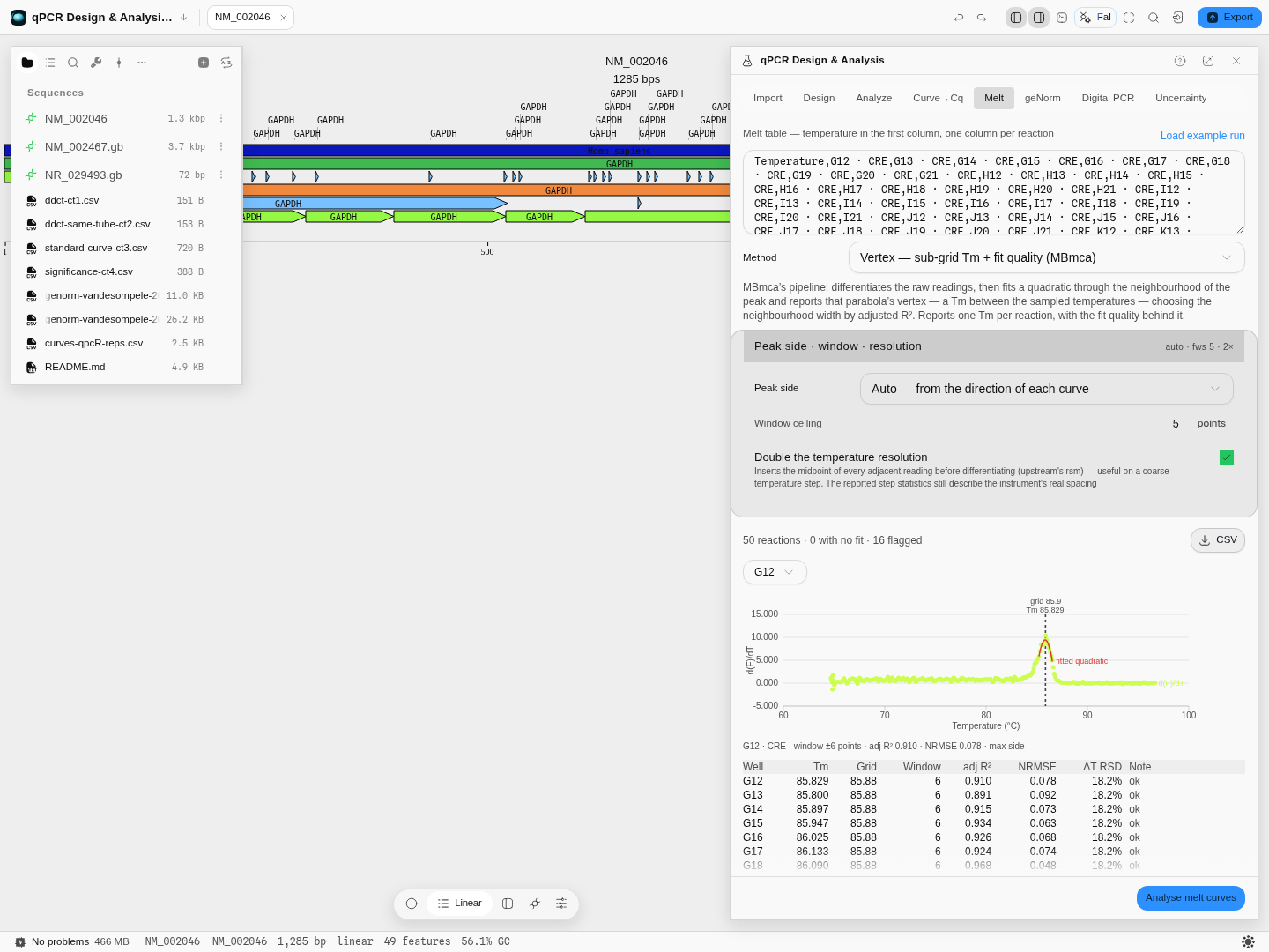
Same well, resolution doubled and the window ceiling dropped to 5: Tm 85.829 against 85.834 — five thousandths of a degree apart, from a fit with a visibly worse adjusted R² (0.910 against 0.989) over a ±6-point window on the doubled grid. The Tm is stable; the fit that produced it is not as good. That is the trade, and you can see both halves of it.
6. Check whether the curves are reproducible at all
Open Replicate spread, below the results. It groups the table's columns by target and reports, at every temperature, the location of the replicates and the spread around it — mean and SD, or median and MAD if one replicate is pulling the group.
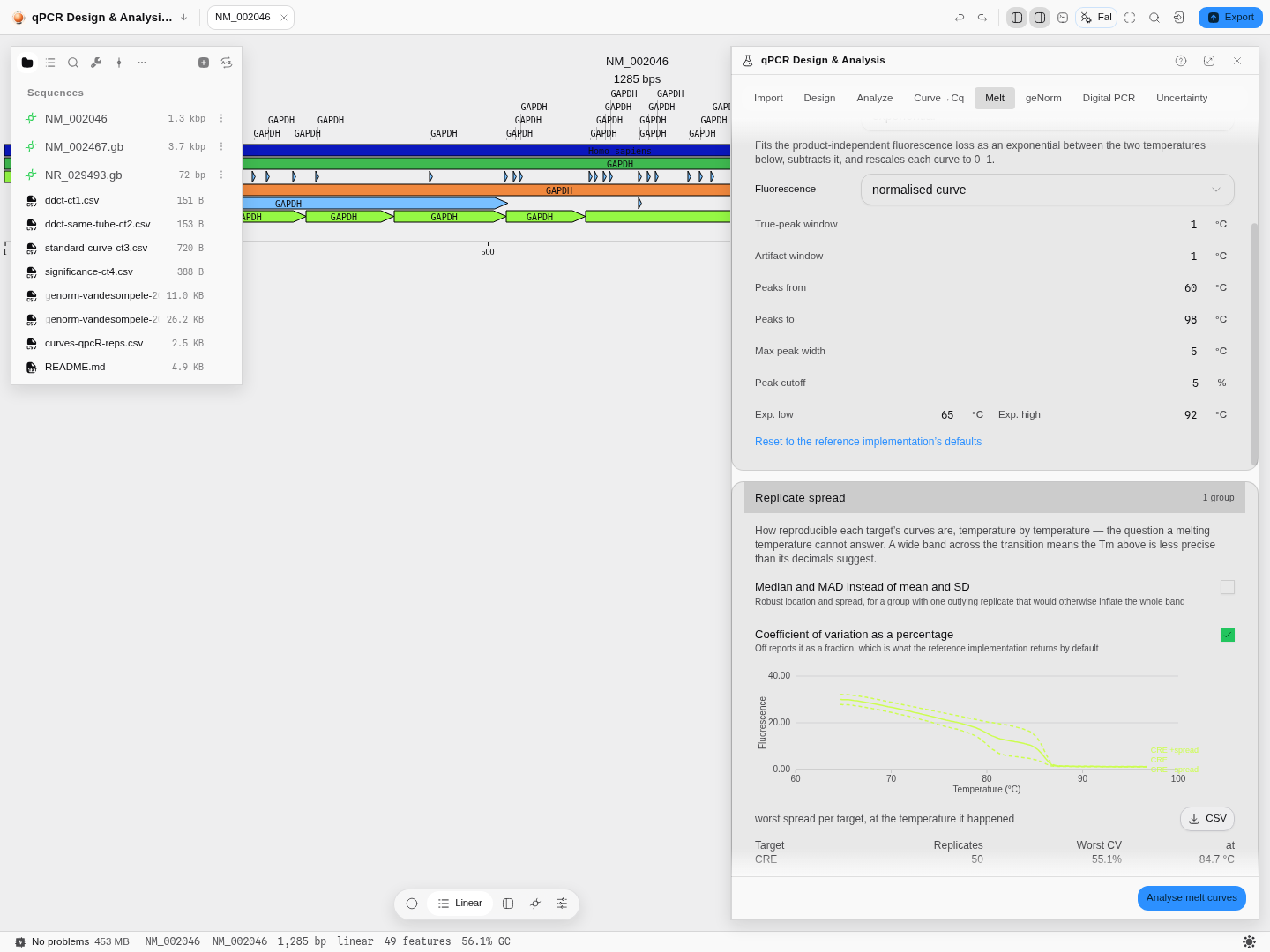
The CRE plate: one target, 50 replicates, worst coefficient of variation 55.1 % at 84.7 °C — half a degree below the product's own melting temperature. That is not a defect in the plate; it is where replicates always diverge, because a small difference in melting behaviour is amplified by the steepest part of the curve. It is also the number that tells you how much of the third decimal on a Tm is real.
A group with one column reports no spread and says so, rather than printing a zero as though it were a measurement.
7. Take the stages away with you
Every stage of the pipeline exports separately — raw, smoothed, normalised, −dF/dT and the second derivative — so you can plot the step you are arguing about rather than the endpoint.
Worked example
Open the qPCR & digital PCR sample project, go to Tools → Melt Curves → Tm and press Load example run. It reads a real 50-reaction melt plate whose CRE target declares an expected melting temperature of 85.34 °C. Press Analyse melt curves.
Forty of the fifty wells come back with a product peak within about a degree of the declared value — mean 85.74 °C. The other ten are named, not dropped.
Now switch the Method selector to the per-curve engine and run it again. It reports 85.77–85.94 °C where the plate engine called 85.66–85.88 °C. Switch once more to the vertex engine: well G12 comes back at 85.834 °C, sub-grid, against a raw grid maximum of 85.99. Three unrelated algorithms, three separate implementations, one answer to within a third of a degree — which is the real reason to have all three. When they disagree, that is information about your curve rather than a bug in one of them.
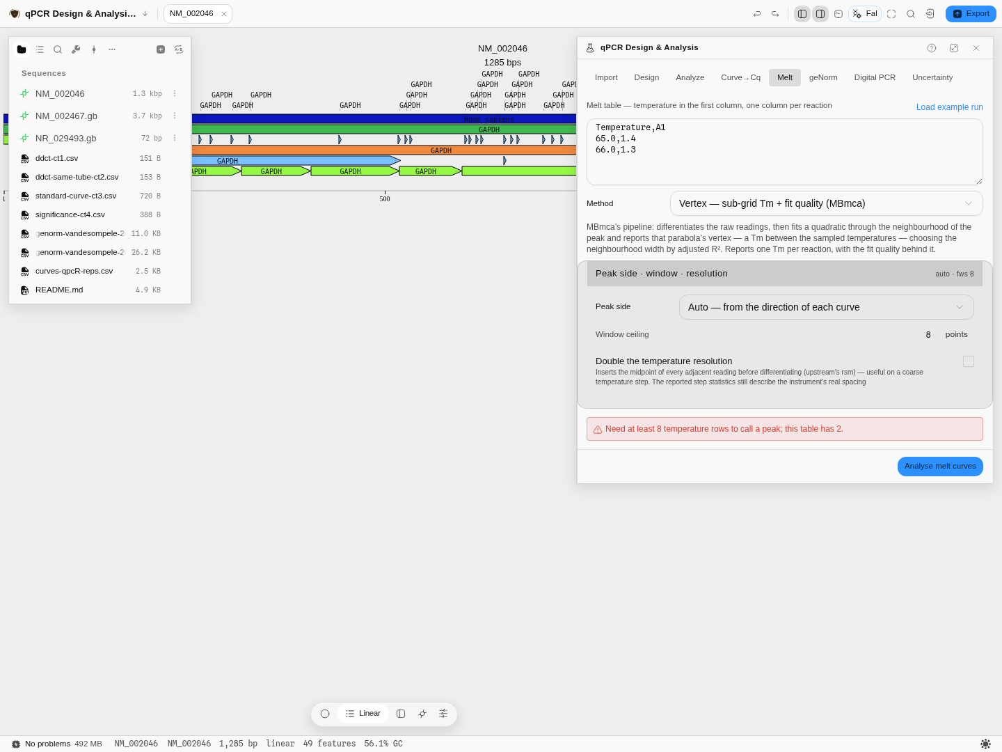
An input the tool cannot use is refused before it runs, with the reason and the count:
Controls
Method — which of the three engines to run (below).
Median and MAD instead of mean and SD, and CV as a percentage — the replicate-spread controls. The robust pair is for a group with one outlying replicate that would otherwise inflate the whole band.
Peak side, window ceiling, double the temperature resolution — the vertex engine's three controls. Peak side decides which end of the derivative the melt sits on (see step 5); the window ceiling bounds how wide a neighbourhood the adjusted-R² search may pick, between 2 and 8 as the reference implementation allows; doubling the resolution inserts midpoints before differentiating.
Normalization — three of them: an exponential fit to the background, a bilinear window scan, or the combination. This is the step that decides what counts as baseline, and it changes peak heights more than it changes peak positions.
Fluorescence source — which channel of the file to read.
Peak band, peak width, fluorescence-drop cutoff — what counts as a peak rather than as noise. A broad shallow bump is primer-dimer or nothing at all depending on where you put these, so they are controls rather than constants.
Expected melting temperature — taken from the file when it states one, and editable when you know better than the file does.
All five pipeline stages have their own download, and the plot draws whichever you select.
Algorithms you can choose
Three engines, and they answer three different questions. This is not one method with a flag.
The plate engine is instrument-grade whole-plate analysis. It normalises, differentiates twice, calls peaks, then classifies each peak against the target's expected temperature — the matching one becomes the product and everything else is grouped into artifact columns shared across the plate. It is the engine that produces verdicts, and it needs the metadata an RDML file carries. Use it to decide whether a run is usable.
The per-curve engine takes one curve at a time and reports every melting peak with the area under it, calling the largest-area peak as the dominant product. No normalisation, no classification, no verdicts. Area is the point: a tall narrow peak and a broad low one can carry the same amount of product, and only the area says so. Use it when you care about the shape of a transition rather than about a pass/fail.
The vertex engine reports a melting temperature that is not one of the temperatures your instrument sampled. Both other engines find the top of a derivative peak and report the temperature of the point sitting there, so their answer can never be finer than your temperature step — on a 0.5 °C ramp, a Tm is quantised to 0.5 °C. This one differentiates the raw readings, then fits a quadratic through the neighbourhood of the peak and reports that parabola's vertex, which lands between the sampled points. It also chooses how wide a neighbourhood to fit by trying every half-width from 2 to your ceiling and keeping the one with the best adjusted R², and it hands you that R², the normalised residual error, and the distance from the raw grid maximum — so the Tm arrives with the evidence for how well it was determined. Use it when you are comparing melting temperatures that differ by less than your temperature step, and when you want a number you can defend.
Underneath the first two, the smoothing is Friedman's super smoother — three fixed spans, a cross-validated per-point choice of span, and that choice itself smoothed — run over the raw curve and again over the first derivative.
The science
Why a derivative. The raw melt curve is a sigmoid falling from fully double-stranded to fully single-stranded, and its steepest point is the melting temperature. Differentiating turns that inflection into a peak, which is far easier to locate and to compare across wells. Differentiating twice locates the peak's own edges, which is how its width and area are measured.
Why normalisation matters, and why it is a choice. Raw fluorescence carries a background that drifts with temperature, and it is not the same background in every well. Subtracting it is unavoidable, and the three methods disagree about what "it" is — an exponential decay, a pair of linear fits either side of the transition, or both. They agree closely on where a peak is and less closely on how tall it is, which is why the tool exposes the choice and shows you the normalised curve rather than only the peak table.
Predicted against measured. The predicted temperature comes from the amplicon's own sequence and salt conditions, by nearest-neighbour thermodynamics. It is a prediction about a defined duplex, not about your tube, so a degree or two of disagreement is normal and a large gap is information — that is why the two numbers sit next to each other instead of one replacing the other.
Provenance. Both engines are checked against the published implementations they follow — 634 reactions across 95,234 temperature points, on two real plates (one that declares an expected temperature and one that does not, because those take different paths), all three normalisations, both fluorescence sources, and every stage of the pipeline including the peak classification itself. Several behaviours that look like defects were confirmed against the reference implementation and kept deliberately, because changing them would silently move every number: the smoother's treatment of the curve ends, the temperature window the bilinear scan actually settles on, and the two different floors used in the two halves of the normalisation. Where the scan's real window differs from the one you asked for, the panel prints the window it used — a control that does not do what its label implies is worse than no control.
Limitations
The second-derivative readout is not implemented. Three engines ship. The published extension that reports the two inflection points either side of a melting peak needs a smoothing spline this tool does not have, and it is queued rather than approximated with a different smoother wearing the same name.
Melt results are not written back into the RDML document. They export as CSV. Round-tripping a file back to instrument software needs a writer this tool does not yet have.
Classification needs an expected temperature. Without one — a bare pasted table, or a file that declares none — you get peaks and areas, not verdicts. That is a real limit and it is stated on screen rather than papered over by promoting the biggest peak.
Keyboard-only and screen-reader operation of this tab has not been verified.
Automation
All three engines are available as one workflow node and to the copilot — analyze_melt_curves.
It takes the same melt table this tab takes, and the engine is a parameter rather than a fixed
choice, so a pipeline can ask for the plate analysis with its verdicts, the sub-grid vertex Tm, or
the per-curve peak areas without opening the tab. Each engine's own controls travel with it: the
window ceiling and extremum side for the vertex engine, the smoothing and area cutoff for the
per-curve one, and the normalisation, peak band, widths and cutoff for the plate.
Two things the node reports that are easy to lose in automation. It names the engine that produced the rows, because a melting temperature without its method is not comparable to one from another method. And when you choose an engine that does not classify, it says so in words — "the vertex engine reports a sub-grid Tm and no verdict" — rather than returning an empty verdict column a script would read as "everything passed".
Replicate spread travels with every run, whichever engine. It describes the readings rather than the method, so it is not hidden behind one engine's selector.
Compared with other tools
Three melt engines, because there are three questions. One does instrument-grade plate analysis and grades every well as product or artifact against the target's own expected Tm; the second measures a single curve's peaks and the area under each, off a spline derivative; the third reports a sub-grid Tm as the vertex of a fitted quadratic, with the fit quality that produced it. Most software offers the first and calls it melt analysis. Having three means a Tm you can cross-check against two unrelated algorithms instead of trusting one implementation — on the bundled CRE plate all three land inside a third of a degree of each other.
A melting temperature finer than your temperature step. Only the vertex engine reports a Tm that is not one of the sampled temperatures, which is what you need when the difference you care about is smaller than the ramp. It comes with an adjusted R², a normalised residual error and the distance from the raw grid maximum, so the number is auditable rather than asserted.
The temperature ramp is measured, not assumed. Every reaction reports the relative spread of its own temperature step, because an uneven ramp moves a melting temperature and nothing else on a instrument report tells you it happened.
Three normalisations, and the intermediate curves. Exponential, bilinear and combined background removal, each selectable — and every stage of the pipeline (raw, smoothed, normalised, −dF/dT, second derivative) is drawable and exportable. Most tools show you the derivative and nothing behind it, which is exactly where a suspicious peak comes from.
Peak calling you control. Window, maximum peak width, area cutoff, true-peak and artifact tolerances, and the expected-Tm range are all fields on the panel, with a one-click return to the reference implementation's defaults.
Peak area, not just peak height. The dominant product is chosen by area, which is the honest way to rank two peaks of different widths.
Measured Tm beside predicted Tm. The Tm computed from the amplicon's own sequence sits next to the one your instrument measured, so "is this the product I designed" is one comparison rather than two tools.
Unclassified stays unclassified. When the file states no expected Tm, every peak is reported without a product identity rather than being assigned one. A verdict invented from nothing is worse than no verdict.
Checked against the reference implementations. All three engines are validated against the published implementations they come from, over their own test corpora — for the vertex engine, that is every curve of every dataset its reference ships: 34 curves, under the default and under each of its switches, with the whole fitted derivative and the chosen window asserted rather than only the Tm.
What it does not do: call a genotype from a high-resolution melt curve, or read proprietary run files with no published schema — bring an RDML export or a temperature/fluorescence table.