
Dot plot
The plot itself, on a pannable canvas with room to read it — the marks, what each engine's marks mean, the run statistics, and a click that selects the matching bases on the sequence.
What it does
A dot plot is a picture of where two sequences agree. One sequence runs along X, the other along Y, and a mark at (i, j) says those two positions matched. Everything you read from a dot plot is a shape: an unbroken diagonal is two sequences that are the same; a diagonal with a gap in it is an insertion or a deletion; a run parallel to the diagonal but offset is a duplicated block; a run on the anti-diagonal is an inversion; a ladder of short parallel runs is a tandem repeat.
This surface is the plot on its own, given the room a shape needs. In a rail-width panel a 20 kb self-comparison is a dense smear; opened on the canvas it pans and zooms, so you can magnify the one place where the diagonal breaks without losing your sense of the whole.
Under the plot sit the run statistics — longest match, longest inverted match, how many matches were drawn in each direction, how much of each sequence is covered, and which substitution matrix scored them when that applies.
When you'd use this
- Comparing a construct against its design. The diagonal shows what matches; the breaks show where your clone is not what you drew.
- Finding repeats before they cost you. A tandem repeat, an inverted repeat, or a duplicated cassette shows here in a form no linear annotation makes obvious — and these are the things that make assemblies collapse and PCRs misprime.
- Placing an unknown contig against a reference before committing to an alignment.
- Seeing a rearrangement. An inversion is an anti-diagonal; a translocation is a block that has moved. An aligner will report these as a pile of numbers; the plot shows them at a glance.
- Comparing two proteins whose identity is low. The matrix-scored engine sees conservative substitutions that exact matching is blind to.
What this computes
Three engines answering three different questions, none subsuming the others, each a port of an
established implementation and checked against it byte for byte including its edge behaviour: the
exact-word (k-mer) plot in the tradition of dottup and FlexiDot, the windowed-identity plot
as seqinr's dotPlot computes it, and the matrix-scored plot as EMBOSS's dotmatcher does. The
legend changes with the engine, because a mark does not mean the same thing.
The statistics EMBOSS prints beside its own plots, in the same order:
- Longest match — the longest run of agreement, in bases or residues. Reported by the two engines that draw runs. The windowed-identity engine draws one mark per window that passed, so it has no run length to measure: it reports the identity bar it applied — how many positions had to agree, out of how many in the window — and the count of windows drawn
- Longest inverted — the longest reverse-complement run, when the reverse pass is on
- Matches drawn — the forward count, and the reverse count when the reverse strand was actually examined. Only the exact-word engine has a reverse-complement pass, and only on a nucleotide comparison with it switched on; otherwise the readout says so rather than printing a zero, because no inverted repeat here and nothing here was looked at are opposite findings and must not share a number
- Scored with — the substitution matrix, for the matrix engine
- Not in the matrix — residues the matrix does not declare, named. They are scored against the matrix's first residue, which is the upstream behaviour kept so the numbers agree; listing them is what stops that being a lie about the score
- Covered — the fraction of X and of Y that any match touches. This is not identity: 40 % coverage means most of that sequence took part in no match at all, whatever the matches look like
- Skipped — windows dropped for exceeding the unknown-residue budget
The unit follows the alphabet: base pairs for nucleotide, residues for protein.
How many of those marks a coin would have drawn. A dot plot is only as meaningful as its word size, and the expected number of chance matches is reported beside the run rather than left implied:
-
Chance matches — how many matching words two unrelated sequences of these lengths would show, under a model in which residues are drawn independently from a background distribution. Two figures are given because they can differ by a lot and each answers a different question. The first uses the composition actually read from your two sequences, so an AT-rich pair is not judged as if its bases were equally likely — on a pair of cricket COI genes the per-position match probability is 0.27, not 0.25, and the expected count is about half as large again. The second assumes a uniform alphabet, which is what the suggested word size is calibrated against, so you can see whether the suggestion is being generous on your particular pair
-
Position pairs compared — how many places a word could have started, which is what the expectation is a count out of
-
Words matched — the observed side: how many matching words this run found on the forward strand, the same unit as the expectation. Runs are not: a 29 bp run holds 24 matching 6 bp words. It is counted before Best path only thins what is drawn
-
Chance windows — the same question for the windowed-identity engine, which marks a window when at least m of its w positions agree. That is a different event from an exact word and takes a different model: the probability that at least m of w independent positions match, counted over the windows the run will really compare under the step and phase you set. It matters most at a loose bar, because a window needing one position in ten to agree passes almost everywhere by chance — the plot fills with marks that mean nothing, and the figure says so before you read them
For those two engines the expectation is combinatorial, not a fitted E-value: both mark under a stated rule, so the count follows from the word or window length and the composition, with no estimated parameters. The exact-word case is the windowed one with every position required to agree, so these are one model read at two settings rather than two that could drift apart.
- Chance marks — the same question for the matrix-scored engine, answered by experiment rather than by formula. A scored mark means "this window's substitution score reached the threshold", and the null distribution of that score depends on the matrix, so there is no combinatorial form to carry over. Instead the run is repeated against a shuffled copy of the second sequence: a permutation keeps its composition exactly and destroys its order, which is the comparison a reader already has in mind — would I see this much if the two were unrelated? The readout gives the marks actually drawn, the mean and standard deviation over the replicates, and the 95th percentile, the count a run has to beat to be surprising at all. Shuffles sets how many replicates; more tightens the estimate and costs one whole plot each. It is seeded, so the figure is reproducible
Read the scored engine's threshold together with that estimate rather than as a significance claim on its own. It is an estimate and says so: unlike the two closed forms it carries a spread, because a mean over replicates without one is a number pretending to be exact.
A reading, generated from the run. Every plot carries a one-sentence finding with the counts and coverage this run produced, then only the cautions this run earned — a chance-match expectation that rivals the number of marks drawn, a self comparison's own leading diagonal, reverse-complement comparison being off so an inversion would leave no mark at all, best-path filtering having removed overlapping matches, words skipped for unknown residues, residues the matrix does not declare — and then the full chain: which engine ran, what it was given, and every policy that applied.
Where it lives
The Dot Plot panel's One-comparison tab draws it in the rail. The plot is also its own surface: detach it as a floating card, or open it as a full canvas tab, where the pan and zoom gestures are. Both are the same component reading the same run, so they cannot show two different plots.
It is part of the editor. Clicking a run selects those bases on the sequence the X axis names — which may not be the document in front of you: the plot's own axis is followed, that document is focused, and only then is the selection made. Coordinates are converted where they need to be, so a plot of a protein record selects the right bases in the underlying sequence rather than the first third of it. If the axis names one record of a multi-sequence file that is not open, that record is opened as its own document first, so a click reaches the bases rather than telling you where to find them. When a run cannot be mapped back — pasted text with no document of its own, a span that does not fit the sequence, or a record that will not open — you are told why, and nothing is selected.
Inputs and outputs
In: two sequences (or one, compared against itself), from the open document, a project file, a selection, or pasted text — chosen in the panel.
Out: the plot, the legend for the engine that produced it, and the statistics EMBOSS prints beside its own plots, in the same order:
| Statistic | What it counts |
|---|---|
| Longest match | The longest run of agreement, in bases or residues — from the two engines that draw runs |
| Identity bar | What the windowed engine required instead: positions that had to agree, out of the window. That engine draws one mark per passing window, so it measures no run length |
| Longest inverted | The longest reverse-complement run, when the reverse pass is on |
| Matches drawn | The forward count, and the reverse count only when the reverse strand was examined. The windowed engine reports windows drawn instead; it and the matrix-scored engine have no reverse-complement pass at all, and the exact-word engine runs one only on a nucleotide pair with Reverse complement on. In every other case the readout says the reverse strand was not examined instead of reporting nought inverted repeats, which would be a different claim |
| Scored with | The substitution matrix, for the matrix engine |
| Not in the matrix | Residues the matrix does not declare, named — they are scored against its first residue rather than being silently dropped |
| Covered | The fraction of X and of Y that any match touches |
| Skipped | Windows dropped for exceeding the unknown-residue budget |
The unit follows the alphabet: base pairs for nucleotide, residues for protein.
Algorithms you can choose
Three engines, and they answer three different questions. None of them subsumes the others, and the legend under the plot changes with the engine because a mark does not mean the same thing:
- Exact word (k-mer). Every exact match of k residues. Fast, crisp, and blind to a diverged repeat — a repeat carrying a substitution every few bases disappears at any useful word size. Blue runs are direct matches, red runs are reverse-complement matches.
- Windowed identity. A window slides along each diagonal and a mark is drawn where the fraction of agreeing positions reaches the threshold. Tolerates mismatches; cannot tell a conservative substitution from a disruptive one.
- Windowed substitution score. The same sliding window, scored through a substitution matrix, with a mark where the score reaches the threshold. This is the one that is right for diverged protein, because it knows that leucine for isoleucine is nearly free and proline for glycine is not.
The matrix follows the alphabet unless you override it — EDNAFULL for DNA, EBLOSUM62 for protein — and you can paste a custom matrix in the standard format.
Worked example
Open the Dot Plot sample project, keep the cricket COI gene Phaneroptera falcata (601 bp) on both axes with Compare with itself on, choose the identity-window method, set Matches required to 9 of a 10 bp window, and plot.
You get the full 601 bp main diagonal — 100% of the sequence covered, 640 matches — plus a scatter of short off-diagonal marks in symmetric pairs. Those pairs are the real finding: a mark at (9, 42) with its mirror at (42, 9) is a repeated 10-mer at two positions in one gene. Click one and the editor selects bases 9–18.
Controls
| Control | What it changes |
|---|---|
| Engine | Which of the three questions above you are asking. |
| Word size (k) | Exact-word engine: the length of match that counts. Larger is stricter and faster. Seeded from the sequence length until you touch it. |
| Window / step | Windowed engines: the length of the window and how far it advances. |
| Threshold | Windowed engines: the identity or score a window must reach. |
| Substitution matrix | Which matrix scores the windows, or a pasted custom one. |
| Reverse complement | Adds the inverted pass, which is what makes inversions and inverted repeats visible. |
| Expand ambiguity codes | Treats IUPAC codes as the bases they stand for rather than as mismatches. |
| Unknown-residue budget | How much of a window may be unknown before the window is skipped — skipped windows are counted and reported. |
| Best path only | Keeps the dominant diagonal rather than every match. |
| Dedupe | Matrix engine: drops the duplicate runs the two passes leave on the shared diagonal. |
| Nucleotide / protein | The alphabet, derived from the input until you set it yourself. |
The science
The engines are ports of the established implementations — the exact-word plot in the tradition of
dottup and FlexiDot, the windowed-identity plot as seqinr's dotPlot computes it, and the
matrix-scored plot as EMBOSS's dotmatcher does — and their matches and coordinates are checked
against those originals byte for byte, including their edge behaviour.
Two details worth knowing because they change what you see:
A residue the matrix does not declare is scored against the matrix's first residue, and named. That is the upstream behaviour, kept so the numbers agree, but silently applying it would be a lie about the score, so the affected residues are listed in the statistics.
Coverage is per axis. Covered reports the fraction of X and of Y that any match touches, which is not the same as identity: a 40% coverage means most of that sequence took part in no match at all, whatever the matches that exist look like.
Limitations
- The exact-word engine is blind to divergence, as above. A blank plot at k = 11 is not evidence of no relationship — lower k, or switch engines, before concluding anything.
- The windowed engines smooth. A single mismatch inside a window that otherwise agrees does not break the mark, which is the point, and it also means a mark is not a claim about every position under it.
- A dot plot is not an alignment. It shows where agreement is; it does not commit to a correspondence, score a gap, or produce coordinates you can hand to a downstream tool. When you need those, align.
- Big comparisons cost. The work grows with the product of the two lengths, and there is a budget that refuses a run rather than hanging — the refusal names the limit and the control that changes it.
Screenshots
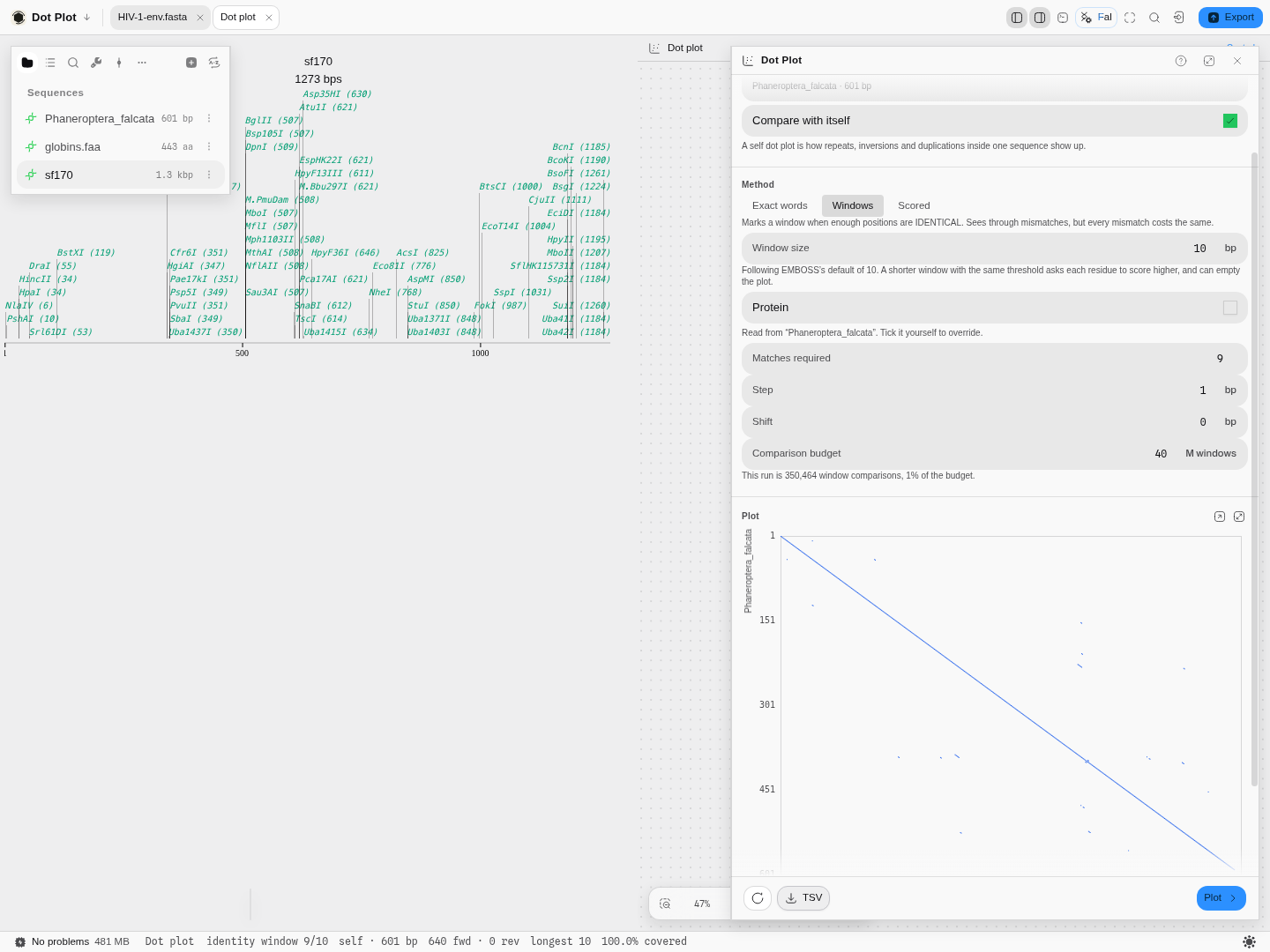 The plot in the rail beneath its controls: a 601 bp self comparison at 9-of-10 identity — the full main diagonal, 100% covered, with the run's cost stated above it.
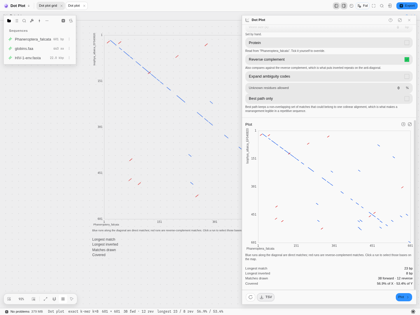 A broken main diagonal — real divergence between two species — with reverse-complement matches drawn in red.
Related
In this group: Edit annotation · Enzyme · Insert sequence · Merge features · Manage enzymes · Dot plot grid · Melt curve · Amplification curves · Population genetics · RNA-seq · Site avoidance heat map · Protein coverage · Reference-gene stability · Digital PCR · Codon usage matrix · Pairwise distance distribution · Nearest-neighbor distances · GC content distribution · Base composition per cycle · Pairwise distance grid · Per-cycle channel occupancy · Grammar assembly plan · Gibson assembly plan · Assembly plan build order · Golden Gate assembly plan · Guide track · Primer binding track · Hydropathy profile · Charge vs pH · Amino-acid composition · Hydrophobic moment · Optimization profiles · Digest gel · Virtual gel · Initiation-window fold · Antibody domain map · Electropherogram · Circuit netlist · Circuit transfer functions · Circuit construct · Construction graph · Protocol · Read Quality Profile · Read Alignment · Raw Signal · Verify vs Reference · Chromosomal microarray · Variant calls · Small molecule