
Pileup viewer
| Document kind | pileup |
| Drawn from | a file — it can also be previewed in the file manager |
| Formats that open here | BAM · SAM |
| Refuses to draw below | 300px wide |
What it draws
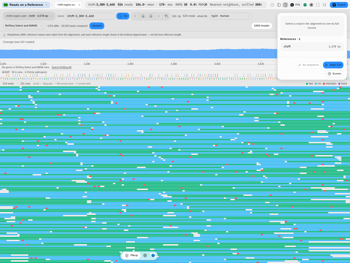
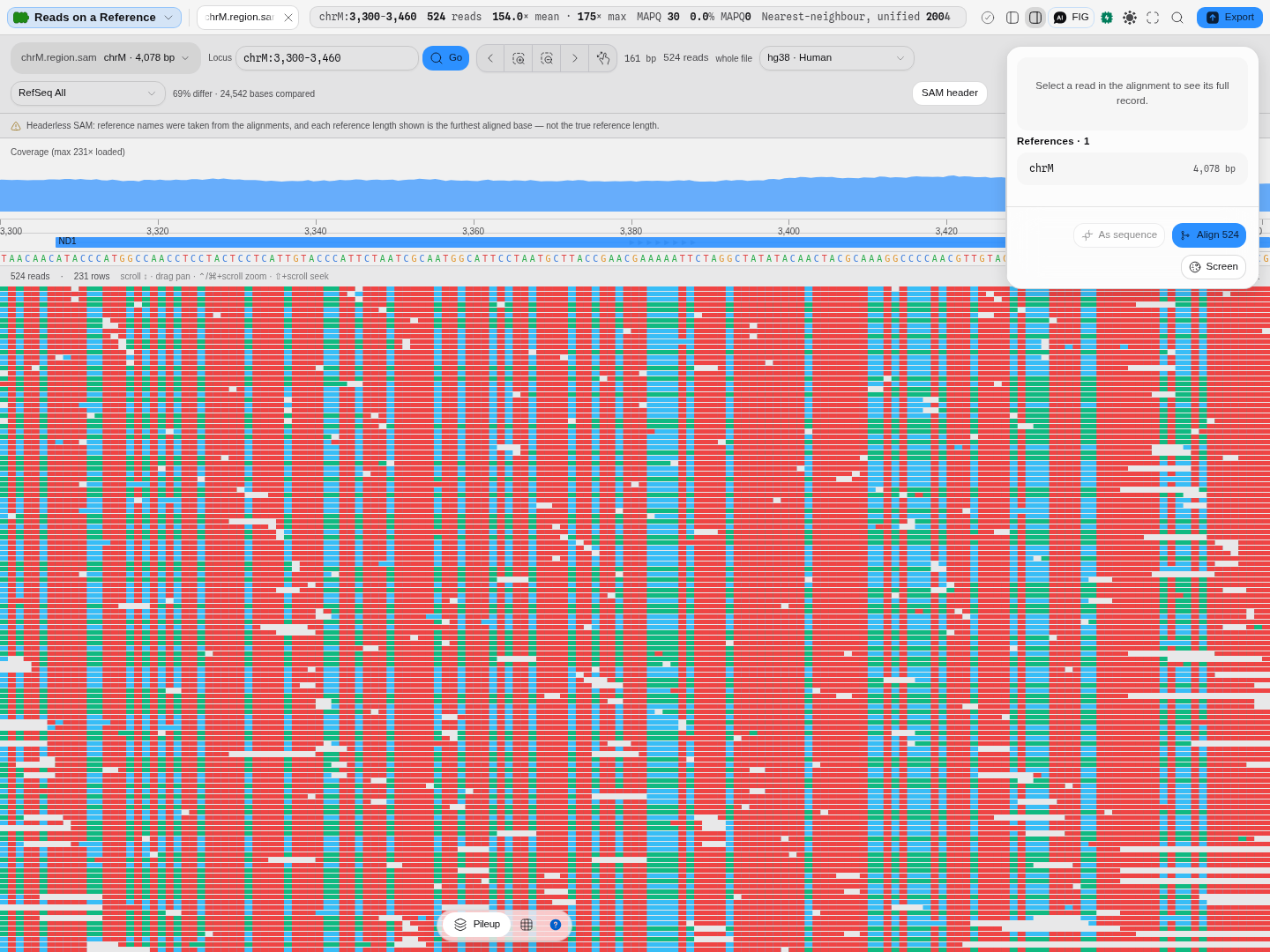
A pileup: every sequencing read that aligned to a window of a reference, stacked so that no two overlapping reads share a row, above a coverage histogram of how deep the alignment is at each position. When a reference sequence is loaded, its bases are drawn under the ruler and the reads carry a mark wherever they disagree with it.
This is the view you use to decide whether a variant is real. A difference supported by two reads out of eighty, all on one strand, at the end of every read, is an artefact — and none of that is visible in a variant table.
What opens in it
BAM and SAM.
A BAM needs its index (.bai or .csi) in the same project. That is not a limitation of this
viewer: a BAM is a compressed, sorted file designed for random access, and without the index there is
no way to find a locus except by reading all of it. IGV and JBrowse require the same thing. The canvas
says so by name rather than drawing an empty window.
A SAM has no index, so it is read whole, which is why the size it accepts is bounded.
A SAM with no header has had its reference dictionary reconstructed from the alignments — and the canvas says so, because the reference lengths it then shows are the furthest aligned base, not the real length of the chromosome. That distinction matters the moment you zoom to fit.
Reads without alignments — a FASTQ — do not open here. They are reads, not a map, and go to the read viewer.
What this computes
Every number this canvas puts on screen, and what it is derived from.
- Depth at each position: how many alignments cover it, counted over every read that overlaps the window rather than over the reads it draws. The histogram is therefore full-depth even where the stack below it is down-sampled.
- Mismatches per read: the positions where the read's base differs from the reference base under
it, found by walking the read's CIGAR against the reference rather than trusting the optional MD
tag most aligners omit. A base the instrument declined to call (
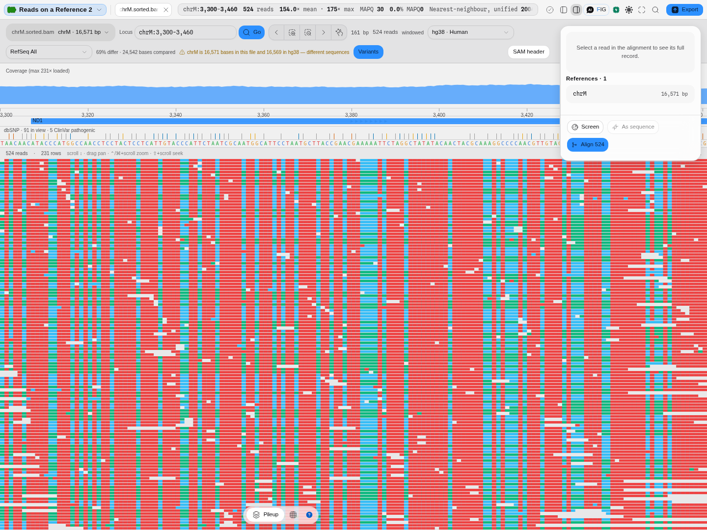
N) is not counted as a mismatch, on either side. That is a deliberate choice and it makes our count differ from the edit distance an aligner writes inNM, which counts a no-call as an edit: a mismatch mark is a claim that the sample carries a different base, and a no-call makes no such claim. - Reference agreement: of the aligned bases in view that had a reference base to compare against, the fraction that differ, reported beside the reference you chose. There is no threshold and no verdict attached to it, because how far a real sample diverges from a reference is the biologist's question and not a constant. Its practical use is immediate: a rate in the tens of percent almost always means the reads were aligned to a different assembly than the one now loaded. Mitochondrial data shows this most sharply, because the older human mitochondrial reference is 16,571 bases and the revised Cambridge reference sequence is 16,569, and an indel near position 310 puts everything downstream out of register.
- Whether the reference is even the right one. An alignment file states the length of each reference it was mapped to, and a reference has a length; when those two numbers differ, the two are not the same sequence, and the viewer says so rather than leaving you to infer it from a high disagreement rate. This is a statement of fact with no threshold behind it — the mitochondrial case is the sharpest: a file mapped to the 16,571-base reference, held against the 16,569-base revised Cambridge sequence, is reported as different sequences however similar the reads look. A length the viewer had to infer — a headerless SAM, where it is the furthest aligned base rather than the reference's real size — is deliberately not compared, because that would manufacture a disagreement out of the file's own caveat.
- Where a reference's reads lie, read from the index alone — no alignment block is fetched to answer it. What can be claimed depends on what the file carries, and the viewer says only what its source supports: a SAM is read whole, so both edges are real and it names the span; a BAI index bounds the RIGHT edge to within one of its own intervals and cannot bound the left at all, so it reports how far the reads REACH and no start; a reference the index holds no intervals for has no reads, and saying so is the point; and a CSI index carries no linear index, so the honest answer there is that it cannot be known. The distinction matters because "no reads on this chromosome" and "this index cannot tell you" look identical on screen and mean completely different things.
- Mapping quality, insert size and pair orientation: read from the alignment record as written. The insert-size band an anomaly is judged against is measured from this alignment's own properly paired reads where there are enough of them, and falls back to a published default where there are not; the canvas says which.
- Gene models under the window, when a public assembly is the reference: transcript bounds, exons and coding bounds exactly as NCBI RefSeq states them, drawn to the convention every genome browser uses (a thin transcript line, medium boxes for untranslated exons, tall ones for coding exons, chevrons for the direction of transcription). You choose which RefSeq set is searched, and the answer depends on it: the curated single-transcript set carries no mitochondrial genes at all, while the curated full set carries the 13 mitochondrial protein-coding genes. An empty track names the set it searched rather than reporting an absence in the locus.
- Known variants under the window, when a public assembly is the reference: dbSNP records with their reference and alternate alleles, dbSNP's own variant class, the highest minor allele frequency any contributing project reports, and whether ClinVar calls the variant pathogenic or benign. The frequency is the highest across projects and is labelled that way, because dbSNP reports one per project and does not say which project each figure came from. Above a couple of thousand marks in one window the track states the count instead of drawing, since a tick per variant stops being a tick.
The variant track is what separates the two readings a red column invites: a mismatch column with an rsID under it is a catalogued variant, and the same column with nothing under it is novel, or an artefact of this library.
Reading it
- Coordinates are 1-based, as in the SAM specification and as in every locus string you paste
(
chr1:1,000,000-1,001,000). - A gap in a read is not a gap in coverage. A read drawn with a thin line through its middle is one alignment spanning a deletion or an intron; a gap between reads is simply no read there.
- Mismatch marks come from the loaded reference where there is one, and fall back to the read's own MD tag where there is not — so a mark is always derived from something the data states rather than guessed. Select a project FASTA as the reference and the marks are against real bases.
- The reference can come from a public assembly instead of a file. Most alignments were made against an assembly nobody keeps a copy of, so the reference picker also lists the assemblies UCSC serves, and fetches the bases for the window you are looking at. Both sources are interchangeable: the same reads over the same window against a project FASTA and against the matching public assembly compare exactly the same bases and report the same disagreement.
- Colour is an encoding you choose. By default it is strand.
- Depth is capped for drawing, not for counting. The read stack is down-sampled above a few thousand rows so the drawing stays responsive, while the coverage track stays full-depth — which is why the histogram can report 900× over a window whose drawn reads you could count.
The misreading this canvas invites most often is taking read colour for a quality judgement. Under the default strand colouring the two colours mean forward and reverse and nothing else. Under insert-size or pair-orientation colouring they mean an anomaly. Read the legend before concluding.
Controls
| Control | What it does |
|---|---|
| Reference | Which sequence in the file's dictionary you are looking at, and optionally a reference to draw real bases and compute mismatches against — either a FASTA in the project, or a public assembly fetched for the window in view. One at a time, so a drawn base always has exactly one source. |
| RefSeq set | Which NCBI RefSeq set the gene models are read from, when a public assembly is the reference. Appears with one. |
| Variants | Turns on the known-variant marks from dbSNP for the window in view. Off until asked for, because it is a third row of marks over the reads. |
| Locus | The window, as a coordinate string. |
| Zoom in / out · Fit | Navigation, clamped at both ends — below the minimum a pileup is a handful of bases; above the maximum it stops being legible and the query gets heavy. |
| Stack | Reads packed into rows, both strands together. |
| Strand stack | Forward reads above the axis, reverse below — the layout for judging strand bias. |
| Paired stack | A read PAIR drawn as one fragment on one row, the two mates joined by the line between them — so an insert is a length you can see rather than two reads you have to associate. |
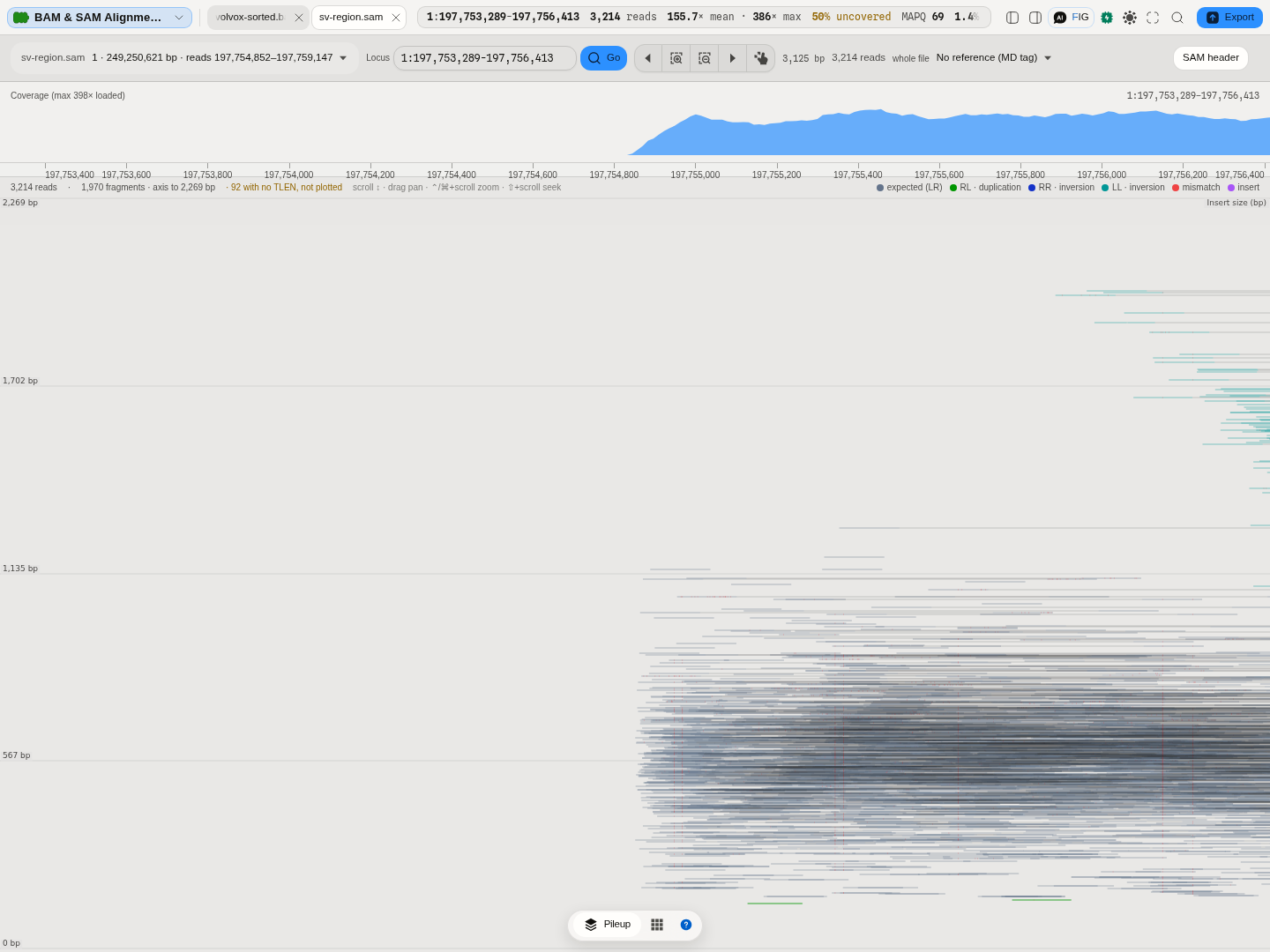
| Inferred size | Every fragment plotted against its own insert size on a value axis, with a log option for a library whose inserts span orders of magnitude. Large inserts sit high; the reads a structural variant leaves behind separate from the main band by height rather than by colour. Fragments the file states no insert size for are counted and left off, and the canvas says how many rather than drawing them at zero. |
| Coverage only | The depth histogram without the reads. |
| Color by | Strand · first-of-pair strand · pair orientation · insert size · insert size and pair orientation · mapping quality · none. Each states what it encodes; the paired modes need a paired-end library. |
| Filter reads | A mapping-quality floor anywhere in the 0-255 range the format allows, and switches to hide secondary, supplementary and duplicate alignments. Nothing is filtered by default, so what you see is what the file says; whatever a filter removes is counted and shown beside the control, because a hidden read is still evidence. The coverage histogram is deliberately not filtered — it answers how deep the data is, not how much of it you chose to draw. |
| Where each reference's reads are | Beside every reference in the picker and the alignment panel. An alignment file's header lists the whole assembly it was mapped against, so a file covering one region still offers you dozens of chromosomes with nothing on them; this says which. |
| Click a read | Its full record — flags, CIGAR, tags, mate, mapping quality. |
All of these are reachable in the preview as well as in the stage tab. A preview has no right-click menu, so the controls are published to the bar rather than living only in the menu.
Where it appears
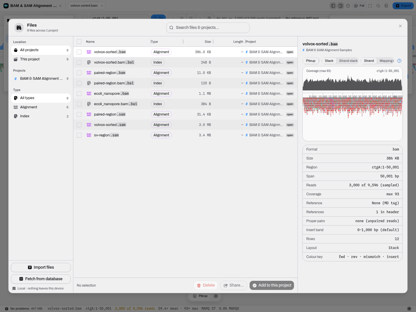
As a stage tab when you open a BAM or SAM, and in the file manager preview. One renderer draws both; the preview has no editor to talk to, so it is read-only navigation.
Export is the editor's one Export panel rather than a button here: the pane publishes its live window, and the panel writes exactly that — reads as TSV, coverage as bedGraph, the window as SAM — alongside the whole alignment.
Screenshots
Performance and limits
- Bytes load lazily on open and are read off the main thread, so a large BAM does not freeze the editor.
- The reads drawn in one window are capped, and the number that actually overlapped is reported, so a down-sampled view says so instead of looking sparse.
- The window span is clamped at both ends, as above.
- It refuses to draw below 300px wide and shows the facts instead. A pileup squeezed narrower is a band of colour in which a cramped alignment and a broken one look identical.
Related
Alignments come from an aligner rather than from this workbench. What the workbench does with them: the Variant calls canvas reads a VCF over the same reference, and the sequence map is where a locus you find here becomes an annotation.